 Hispanopedia Wiki
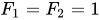
En matemáticas, la sucesión de Fibonacci es una sucesión en la que cada elemento es la suma de los dos elementos que lo preceden. Los números que forman parte de la sucesión de Fibonacci se conocen como números de Fibonacci , comúnmente denotados F n . Los elementos iniciales de la sucesión son F 1 = 1 y F 2 = 1 , aunque muchos autores también incluyen un elemento cero F 0 = 0 . [ 1 ] [ 2 ] Partiendo de F 0 , la sucesión comienza

Los números de Fibonacci fueron descritos por primera vez en las matemáticas indias ya en el año 200 a. C. en la obra de Pingala sobre la enumeración de posibles patrones de poesía sánscrita formados a partir de sílabas de dos longitudes. [ 3 ] [ 4 ] [ 5 ] Reciben su nombre del matemático italiano Leonardo de Pisa, también conocido como Fibonacci , quien introdujo la secuencia en las matemáticas de Europa occidental en su libro Liber Abaci de 1202. [ 6 ]
Los números de Fibonacci aparecen con una frecuencia inesperada en matemáticas, hasta el punto de que existe una revista dedicada exclusivamente a su estudio, la Fibonacci Quarterly . Entre las aplicaciones de los números de Fibonacci se incluyen algoritmos informáticos como la técnica de búsqueda de Fibonacci y la estructura de datos de montón de Fibonacci , así como grafos denominados cubos de Fibonacci, utilizados para interconectar sistemas paralelos y distribuidos. También aparecen en contextos biológicos , como la ramificación de los árboles, la disposición de las hojas en un tallo , los brotes de la piña , la floración de la alcachofa y la disposición de las brácteas de una piña de pino , aunque no se dan en todas las especies.
Fibonacci numbers are also strongly related to the golden ratio: Binet's formula expresses the n-th Fibonacci number in terms of n and the golden ratio, and implies that the ratio of two consecutive Fibonacci numbers tends to the golden ratio as n increases. Fibonacci numbers are also closely related to Lucas numbers, which obey the same recurrence relation and with the Fibonacci numbers form a complementary pair of Lucas sequences.
Definition

The Fibonacci numbers may be defined by the recurrence relation[7] and for n > 1.


Under some older definitions, the value is omitted, so that the sequence starts with .[8][9]

The first 21 Fibonacci numbers Fn are:
The Fibonacci sequence can be extended to negative integer indices by following the same recurrence relation in the negative direction (sequence A039834 in the OEIS): , , and for n < 0 . Nearly all properties of Fibonacci numbers do not depend upon whether the indices are positive or negative. The values for positive and negative indices obey the relation:[10]



History
India

La secuencia de Fibonacci aparece en las matemáticas indias , en relación con la prosodia sánscrita . [ 4 ] [ 11 ] [ 12 ] En la tradición poética sánscrita, existía interés en enumerar todos los patrones de sílabas largas (L) de 2 unidades de duración, yuxtapuestas con sílabas cortas (S) de 1 unidad de duración. Contando los diferentes patrones de L y S sucesivas con una duración total dada se obtienen los números de Fibonacci: el número de patrones de duración m unidades es F m +1 . [ 5 ]
El conocimiento de la secuencia de Fibonacci se expresó ya en Pingala ( c. 450 a. C.–200 a. C.). Singh cita la fórmula críptica de Pingala misrau cha ("los dos están mezclados") y a los eruditos que la interpretan en contexto como diciendo que el número de patrones para m tiempos ( F m +1 ) se obtiene añadiendo un [S] a los casos F m y un [L] a los casos F m −1 . [ 13 ] Bharata Muni también expresa conocimiento de la secuencia en el Natya Shastra ( c. 100 a. C.–c. 350 d . C.). [ 3 ] [ 4 ] Sin embargo, la exposición más clara de la secuencia surge en la obra de Virahanka ( c. 700 d. C.), cuya propia obra se ha perdido, pero está disponible en una cita de Gopala ( c. 1135): [ 12 ]
Variaciones de dos metros anteriores [es la variación] ... Por ejemplo, para [un metro de longitud] cuatro, al mezclarse variaciones de metros de dos [y] tres, se obtiene cinco. [resuelve los ejemplos 8, 13, 21] ... De esta manera, el proceso debe seguirse en todas las mātrā-vṛttas [combinaciones prosódicas]. [ a ]
A Hemachandra ( c. 1150) también se le atribuye el conocimiento de la secuencia, [ 3 ] escribiendo que "la suma del último y el anterior es el número ... del siguiente mātrā-vṛtta". [ 15 ] [ 16 ]
Europa

La secuencia de Fibonacci aparece por primera vez en el libro Liber Abaci ( El Libro de Cálculos , 1202) de Fibonacci , [ 17 ] [ 18 ] donde se utiliza para calcular el crecimiento de poblaciones de conejos. [ 19 ] Fibonacci considera el crecimiento de una población de conejos idealizada ( biológicamente irreal) , asumiendo que: una pareja reproductora recién nacida se coloca en un campo; cada pareja reproductora se aparea a la edad de un mes, y al final de su segundo mes siempre producen otra pareja de conejos; y los conejos nunca mueren, sino que continúan reproduciéndose para siempre. Fibonacci planteó el problema matemático del conejo : ¿cuántas parejas habrá en un año?
- Al final del primer mes, se aparean, pero sigue habiendo solo una pareja.
- Al final del segundo mes, producen una nueva pareja, por lo que hay 2 parejas en el campo.
- Al final del tercer mes, la pareja original produce una segunda pareja, pero esta segunda pareja solo se aparea para gestar durante un mes, por lo que hay 3 parejas en total.
- Al final del cuarto mes, la pareja original ha producido otra nueva pareja, y la pareja nacida hace dos meses también produce su primera pareja, con lo que suma 5 parejas.
Al final del n -ésimo mes, el número de parejas de conejos es igual al número de parejas maduras (es decir, el número de parejas en el mes n – 2 ) más el número de parejas vivas el mes anterior (mes n – 1 ). El número en el n -ésimo mes es el n -ésimo número de Fibonacci. [ 20 ]
El nombre "secuencia de Fibonacci" fue utilizado por primera vez por el teórico de números del siglo XIX Édouard Lucas . [ 21 ]

Relación con la proporción áurea
Expresión en forma cerrada
Like every sequence defined by a homogeneous linear recurrence with constant coefficients, the Fibonacci numbers have a closed-form expression.[22] It has become known as Binet's formula, named after French mathematician Jacques Philippe Marie Binet, though it was already known by Abraham de Moivre and Daniel Bernoulli:[23]
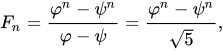
where (phi) is the golden ratio and (psi) is its conjugate,[24]


![{\displaystyle {\begin{aligned}\varphi &={\tfrac {1}{2}}{\bigl (}1+{\sqrt {5}}~\!{\bigr )}={\phantom {-}}1.61803\ldots ,\\[5mu]\psi &={\tfrac {1}{2}}{\bigl (}1-{\sqrt {5}}~\!{\bigr )}=-0.61803\ldots .\end{aligned}}}](https://wikimedia.org/api/rest_v1/media/math/render/svg/fa482a39307037a76b9ae70dd5e1eaa11918e98f)

The numbers and are the two solutions of the quadratic equation, that is, , and thus they satisfy the identities and .


Since , Binet's formula can also be written as


To see the relation between the sequence and these constants,[25] note that and are also roots of so the powers of and satisfy the Fibonacci recurrence. In other words,

![{\displaystyle {\begin{aligned}\varphi ^{n}&=\varphi ^{n-1}+\varphi ^{n-2},\\[3mu]\psi ^{n}&=\psi ^{n-1}+\psi ^{n-2}.\end{aligned}}}](https://wikimedia.org/api/rest_v1/media/math/render/svg/282a0b620cb2eca72787ef444e6d07d39678d383)
It follows that for any values a and b, the sequence defined by

satisfies the same recurrence. If a and b are chosen so that U0 = 0 and U1 = 1 then the resulting sequence Un must be the Fibonacci sequence. This is the same as requiring a and b satisfy the system of equations:

which has solution
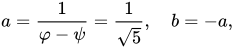
producing the required formula.
Taking the starting values U0 and U1 to be arbitrary constants and solving the system of equations gives the general solution In particular, choosing a = 1 makes the n-th element of the sequence closely approximate the n-th power of for large enough values of n. This arises when U0 = 2 and U1 = 1, which produces the sequence of Lucas numbers.
![{\displaystyle {\begin{aligned}a&={\frac {U_{1}-U_{0}\psi }{\sqrt {5}}},\\[3mu]b&={\frac {U_{0}\varphi -U_{1}}{\sqrt {5}}}.\end{aligned}}}](https://wikimedia.org/api/rest_v1/media/math/render/svg/9b7a1f5df3f3d8a6b6e48e76a19c75a2b5c65645)
Computation by rounding
Since for all n ≥ 0, the number Fn is the closest integer to . Therefore, it can be found by rounding, using the nearest integer function:


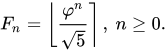
In fact, the rounding error quickly becomes very small as n grows, being less than 0.1 for n ≥ 4, and less than 0.01 for n ≥ 8. This formula is easily inverted to find an index of a Fibonacci number F:

Instead using the floor function gives the largest index of a Fibonacci number that is not greater than F: where , ,[26] and .[27]




Magnitude
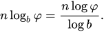
Since Fn is asymptotic to , the number of digits in Fn is asymptotic to . As a consequence, for every integer d > 1 there are either 4 or 5 Fibonacci numbers with d decimal digits.


More generally, in the baseb representation, the number of digits in Fn is asymptotic to
Limit of consecutive quotients
Johannes Kepler observed that the ratio of consecutive Fibonacci numbers converges. He wrote that "as 5 is to 8 so is 8 to 13, practically, and as 8 is to 13, so is 13 to 21 almost", and concluded that these ratios approach the golden ratio :[28][29]
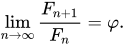
This convergence holds regardless of the starting values and , unless . This can be verified using Binet's formula. For example, the initial values 3 and 2 generate the sequence 3, 2, 5, 7, 12, 19, 31, 50, 81, 131, 212, 343, 555, .... The ratio of consecutive elements in this sequence shows the same convergence towards the golden ratio.


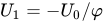
In general, , because the ratios between consecutive Fibonacci numbers approaches .
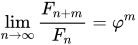

Successive tilings of the plane and a graph of approximations to the golden ratio calculated by dividing each Fibonacci number by the previous
Decomposition of powers
Since the golden ratio satisfies the equation

this expression can be used to decompose higher powers as a linear function of lower powers, which in turn can be decomposed all the way down to a linear combination of and 1. The resulting recurrence relationships yield Fibonacci numbers as the linear coefficients: Esta ecuación se puede demostrar por inducción sobre n ≥ 1 : Para, también es cierto quey también es cierto que





Estas expresiones también son válidas para n < 1 si la secuencia de Fibonacci F n se extiende a enteros negativos utilizando la regla de Fibonacci.

Identificación
La fórmula de Binet proporciona una prueba de que un entero positivo x es un número de Fibonacci si y solo si al menos uno deoes un cuadrado perfecto . [ 30 ] Esto se debe a que la fórmula de Binet, que se puede escribir como, se puede multiplicar pory resuelta como una ecuación cuadrática enmediante la fórmula cuadrática :





Comparando esto conDe ello se deduce que


En particular, el lado izquierdo es un cuadrado perfecto.
Forma matricial
Un sistema bidimensional de ecuaciones en diferencias lineales que describe la secuencia de Fibonacci es
alternativamente denominado

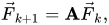
lo cual produceLos valores propios de la matriz A sonycorrespondientes a los respectivos autovectores

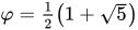


Como el valor inicial es De ello se deduce que el n- ésimo elemento es


A partir de esto, el enésimo elemento de la secuencia de Fibonacci se puede leer directamente como una expresión de forma cerrada :

De forma equivalente, el mismo cálculo puede realizarse diagonalizando A mediante el uso de su descomposición en valores propios : dónde Por lo tanto, la expresión en forma cerrada para el n -ésimo elemento de la secuencia de Fibonacci viene dada por: lo que nuevamente produce
![{\displaystyle {\begin{aligned}A&=S\Lambda S^{-1},\\[3mu]A^{n}&=S\Lambda ^{n}S^{-1},\end{aligned}}}](https://wikimedia.org/api/rest_v1/media/math/render/svg/2fba6879ab00e30ad2d346663f77b8945d261b71)


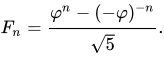
La matriz A tiene un determinante de −1, y por lo tanto es una matriz unimodular de 2 × 2 .
Esta propiedad puede entenderse en términos de la representación en fracción continua de la proporción áurea φ : The convergents of the continued fraction for φ are ratios of successive Fibonacci numbers: φn = Fn+1 / Fn is the n-th convergent, and the (n + 1)-st convergent can be found from the recurrence relation φn+1 = 1 + 1 / φn.[31] The matrix formed from successive convergents of any continued fraction has a determinant of +1 or −1. The matrix representation gives the following closed-form expression for the Fibonacci numbers: For a given n, this matrix can be computed in O(log n) arithmetic operations,[b] using the exponentiation by squaring method.
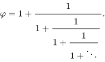
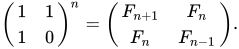
Taking the determinant of both sides of this equation yields Cassini's identity,

Moreover, since AnAm = An+m for any square matrixA, the following identities can be derived (they are obtained from two different coefficients of the matrix product, and one may easily deduce the second one from the first one by changing n into n + 1),
![{\displaystyle {\begin{aligned}{F_{m}}{F_{n}}+{F_{m-1}}{F_{n-1}}&=F_{m+n-1},\\[3mu]F_{m}F_{n+1}+F_{m-1}F_{n}&=F_{m+n}.\end{aligned}}}](https://wikimedia.org/api/rest_v1/media/math/render/svg/9759138bd138ff200cb7ce83c6585d4b0a05b5a1)
In particular, with m = n,
![{\displaystyle {\begin{aligned}F_{2n-1}&={F_{n}}^{2}+{F_{n-1}}^{2}\\[6mu]F_{2n{\phantom {{}-1}}}&=(F_{n-1}+F_{n+1})F_{n}\\[3mu]&=(2F_{n-1}+F_{n})F_{n}\\[3mu]&=(2F_{n+1}-F_{n})F_{n}.\end{aligned}}}](https://wikimedia.org/api/rest_v1/media/math/render/svg/c52b4967a19817553ce67e6d0ff1d411d4141731)
These last two identities provide a way to compute Fibonacci numbers recursively in O(log n) arithmetic operations. This matches the time for computing the n-th Fibonacci number from the closed-form matrix formula, but with fewer redundant steps if one avoids recomputing an already computed Fibonacci number (recursion with memoization).[32]
Combinatorial identities
Combinatorial proofs
Most identities involving Fibonacci numbers can be proved using combinatorial arguments using the fact that can be interpreted as the number of (possibly empty) sequences of 1s and 2s whose sum is . This can be taken as the definition of with the conventions , meaning no such sequence exists whose sum is −1, and , meaning the empty sequence "adds up" to 0. In the following, is the cardinality of a set:


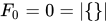





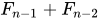
In this manner the recurrence relation puede entenderse dividiendo elsecuencias en dos conjuntos que no se superponen, donde todas las secuencias comienzan con 1 o 2: Excluyendo el primer elemento, los términos restantes en cada secuencia sumanoy la cardinalidad de cada conjunto esodando un total desecuencias, mostrando que esto es igual a.



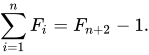
De manera similar se puede demostrar que la suma de los primeros números de Fibonacci hasta el n -ésimo es igual al ( n + 2) -ésimo número de Fibonacci menos 1. [ 33 ] En símbolos:
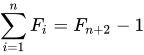
Esto se puede observar dividiendo todas las secuencias que sumanbasado en la ubicación de los dos primeros. Específicamente, cada conjunto consta de aquellas secuencias que comienzanhasta los dos últimos setscada uno con cardinalidad 1.



Siguiendo la misma lógica que antes, al sumar la cardinalidad de cada conjunto vemos que

... donde los dos últimos términos tienen el valorDe esto se deduce que.
Un argumento similar, agrupando las sumas por la posición del primer 1 en lugar del primer 2, da dos identidades más: y En palabras, la suma de los primeros números de Fibonacci con índice impar hastaes el (2 n ) -ésimo número de Fibonacci, y la suma de los primeros números de Fibonacci con índice par hastaes el (2 n + 1) -ésimo número de Fibonacci menos 1. [ 34 ]
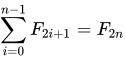
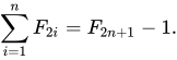


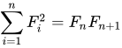
Se puede utilizar otro truco para demostrarlo. o en palabras, la suma de los cuadrados de los primeros números de Fibonacci hastaes el producto de los números de Fibonacci n -ésimo y ( n + 1) -ésimo. Para ver esto, comencemos con un rectángulo de Fibonacci de tamañoy descomponerlo en cuadrados de tamaño; a partir de esto, la identidad se deduce comparando áreas:


Pruebas por inducción
Las identidades de Fibonacci a menudo se pueden demostrar fácilmente utilizando la inducción matemática .
Por ejemplo, reconsiderar Agregara ambas partes da

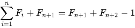
y así tenemos la fórmula para
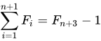
De manera similar, agreguea ambos lados de dar


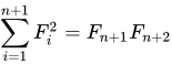
Demostraciones de fórmulas de Binet
La fórmula de Binet es Esto puede utilizarse para demostrar identidades de Fibonacci.

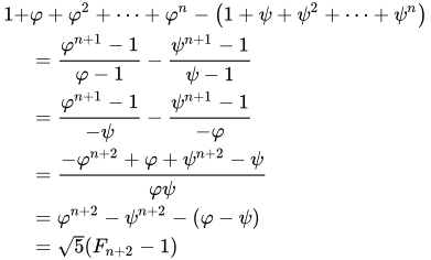
Por ejemplo, para demostrar que tenga en cuenta que el lado izquierdo multiplicado porse convierte según sea necesario, utilizando los hechos.ypara simplificar las ecuaciones.




Otras identidades
Se pueden derivar numerosas otras identidades utilizando diversos métodos. Aquí hay algunos de ellos: [ 35 ]
Las identidades de Cassini y Catalán
La identidad de Cassini afirma que La identidad catalana es una generalización:


La identidad de d'Ocagne
donde L n es el n - ésimo número de Lucas . El último es una identidad para duplicar n ; otras identidades de este tipo son por la identidad de Cassini.



These can be found experimentally using lattice reduction, and are useful in setting up the special number field sieve to factorize a Fibonacci number.



More generally,[35]

or alternatively

Putting k = 2 in this formula, one gets again the formulas of the end of above section Matrix form.
Generating functions
Ordinary
The ordinary generating function of the Fibonacci sequence is the power series

This series is convergent for any complex number satisfying and its sum has a simple closed form:[36]


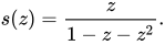
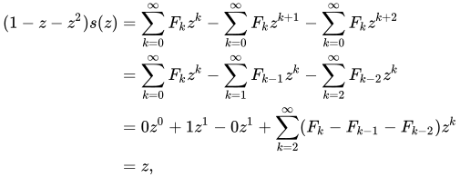
This can be proved by multiplying by : where all terms involving for cancel out because of the defining Fibonacci recurrence relation.



Using lays out the Fibonacci numbers through the second-last number with digits in the decimal expansion of . For example,


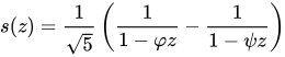
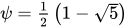
The partial fraction decomposition is given by where is the golden ratio and is its conjugate.

Exponential
The exponential generating function of the Fibonacci sequence may also be derived from the recurrence relation, giving a homogeneouslinear differential equation: The characteristic polynomial of this equation is , to which the solutions are exactly the golden ratio and its conjugate. Combined with the initial values and , the exponential generating function of the Fibonacci numbers is given by the entire function Evaluating the derivatives of the exponential generating function at gives Binet's formula:


Reciprocal sums
Infinite sums over reciprocal Fibonacci numbers can sometimes be evaluated in terms of theta functions. For example, the sum of every odd-indexed reciprocal Fibonacci number can be written as
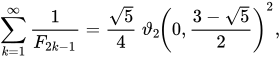
and the sum of squared reciprocal Fibonacci numbers as

If we add 1 to each Fibonacci number in the first sum, there is also the closed form
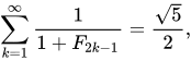
and there is a nested sum of squared Fibonacci numbers giving the reciprocal of the golden ratio,
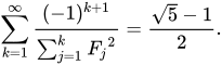
The sum of all even-indexed reciprocal Fibonacci numbers is[37] with the Lambert series since
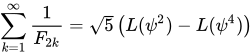
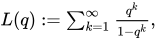
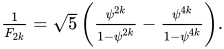
So the reciprocal Fibonacci constant is[38]

Moreover, this number has been proved irrational by Richard André-Jeannin.[39]
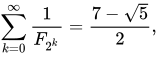
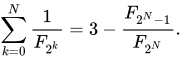
Millin's series gives the identity[40] which follows from the closed form for its partial sums as N tends to infinity:
Primes and divisibility
Divisibility properties
Every third number of the sequence is even (a multiple of ) and, more generally, every -th number of the sequence is a multiple of . Thus the Fibonacci sequence is an example of a divisibility sequence. In fact, the Fibonacci sequence satisfies the stronger divisibility property[41][42] where gcd is the greatest common divisor function. (This relation is different if a different indexing convention is used, such as the one that starts the sequence with and .)




In particular, any three consecutive Fibonacci numbers are pairwise coprime because both and . That is, for every n.


Every prime numberp divides a Fibonacci number that can be determined by the value of pmodulo 5. If p is congruent to 1 or 4 modulo 5, then p divides Fp−1, and if p is congruent to 2 or 3 modulo 5, then, p divides Fp+1. The remaining case is that p = 5, and in this case p divides Fp.
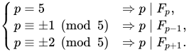
These cases can be combined into a single, non-piecewise formula, using the Legendre symbol:[43]

Primality testing
The above formula can be used as a primality test in the sense that if where the Legendre symbol has been replaced by the Jacobi symbol, then this is evidence that n is a prime, and if it fails to hold, then n is definitely not a prime. If n is composite and satisfies the formula, then n is a Fibonacci pseudoprime. When m is large –say a 500-bit number –then we can calculate Fm (mod n) efficiently using the matrix form. Thus

Here the matrix power Am is calculated using modular exponentiation, which can be adapted to matrices.[44]

Fibonacci primes
A Fibonacci prime is a Fibonacci number that is prime. The first few are:[45]
- 2, 3, 5, 13, 89, 233, 1597, 28657, 514229, ...
Fibonacci primes with thousands of digits have been found, but it is not known whether there are infinitely many.[46]
Fkn is divisible by Fn, so, apart from F4 = 3, any Fibonacci prime must have a prime index. As there are arbitrarily long runs of composite numbers, there are therefore also arbitrarily long runs of composite Fibonacci numbers.
No Fibonacci number greater than F6 = 8 is one greater or one less than a prime number.[47]
The only nontrivial square Fibonacci number is 144.[48] Attila Pethő proved in 2001 that there is only a finite number of perfect power Fibonacci numbers.[49] In 2006, Y. Bugeaud, M. Mignotte, and S. Siksek proved that 8 and 144 are the only such non-trivial perfect powers.[50]
The only triangular Fibonacci numbers are 1, 3, 21, and 55, which was conjectured by Vern Hoggatt and proved by Luo Ming.[51]
No Fibonacci number can be a perfect number.[52] More generally, no Fibonacci number other than 1 can be multiply perfect,[53] and no ratio of two Fibonacci numbers can be perfect.[54]
Prime divisors
With the exceptions of 1, 8 and 144 (F1 = F2, F6 and F12) every Fibonacci number has a prime factor that is not a factor of any smaller Fibonacci number (Carmichael's theorem).[55] As a result, 8 and 144 (F6 and F12) are the only Fibonacci numbers that are the product of other Fibonacci numbers.[56]
The divisibility of Fibonacci numbers by a prime p is related to the Legendre symbol which is evaluated as follows:

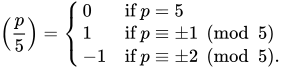
If p is a prime number then [57][58]

For example,

It is not known whether there exists a prime p such that

Such primes (if there are any) would be called Wall–Sun–Sun primes.
Also, if p ≠ 5 is an odd prime number then:[59]

Example 1.p = 7, in this case p ≡ 3 (mod 4) and we have:



Example 2.p = 11, in this case p ≡ 3 (mod 4) and we have:



Example 3.p = 13, in this case p ≡ 1 (mod 4) and we have:



Example 4.p = 29, in this case p ≡ 1 (mod 4) and we have:



For odd n, all odd prime divisors of Fn are congruent to 1 modulo 4, implying that all odd divisors of Fn (as the products of odd prime divisors) are congruent to 1 modulo 4.[60]
For example,

All known factors of Fibonacci numbers F(i) for all i < 50000 are collected at the relevant repositories.[61][62]
Periodicity modulo n
If the members of the Fibonacci sequence are taken mod n, the resulting sequence is periodic with period at most 6n.[63] The lengths of the periods for various n form the so-called Pisano periods.[64] Determining a general formula for the Pisano periods is an open problem, which includes as a subproblem a special instance of the problem of finding the multiplicative order of a modular integer or of an element in a finite field. However, for any particular n, the Pisano period may be found as an instance of cycle detection.
Generalizations
The Fibonacci sequence is one of the simplest and earliest known sequences defined by a recurrence relation, and specifically by a linear difference equation. All these sequences may be viewed as generalizations of the Fibonacci sequence. In particular, Binet's formula may be generalized to any sequence that is a solution of a homogeneous linear difference equation with constant coefficients.
Some specific examples that are close, in some sense, to the Fibonacci sequence include:
- Generalizing the index to negative integers to produce the negafibonacci numbers.
- Generalizing the index to real numbers using a modification of Binet's formula.[35]
- Starting with other integers. Lucas numbers have L1 = 1, L2 = 3, and Ln = Ln−1 + Ln−2. Primefree sequences use the Fibonacci recursion with other starting points to generate sequences in which all numbers are composite.
- Letting a number be a linear function (other than the sum) of the 2 preceding numbers. The Pell numbers have Pn = 2Pn−1 + Pn−2. If the coefficient of the preceding value is assigned a variable value x, the result is the sequence of Fibonacci polynomials.
- Not adding the immediately preceding numbers. The Padovan sequence and Perrin numbers have P(n) = P(n − 2) + P(n − 3).
- Generating the next number by adding 3 numbers (tribonacci numbers), 4 numbers (tetranacci numbers), or more. The resulting sequences are known as k-Step Fibonacci numbers.[65] They are also commonly referred to as k-bonacci numbers.[66]
Applications
Mathematics

The Fibonacci numbers occur as the sums of binomial coefficients in the "shallow" diagonals of Pascal's triangle:[67] This can be proved by expanding the generating function and collecting like terms of .
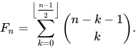


To see how the formula is used, we can arrange the sums by the number of terms present:
which is , where we are choosing the positions of k twos from n−k−1 terms.


These numbers also give the solution to certain enumerative problems,[68] the most common of which is that of counting the number of ways of writing a given number n as an ordered sum of 1s and 2s (called compositions); there are Fn+1 ways to do this (equivalently, it's also the number of domino tilings of the rectangle). For example, there are F5+1 = F6 = 8 ways one can climb a staircase of 5 steps, taking one or two steps at a time:

The figure shows that 8 can be decomposed into 5 (the number of ways to climb 4 steps, followed by a single-step) plus 3 (the number of ways to climb 3 steps, followed by a double-step). The same reasoning is applied recursively until a single step, of which there is only one way to climb.
The Fibonacci numbers can be found in different ways among the set of binarystrings, or equivalently, among the subsets of a given set.
- El número de cadenas binarias de longitud n sin unos consecutivos es el número de Fibonacci F n +2 . Por ejemplo, de las 16 cadenas binarias de longitud 4, hay F 6 = 8 sin unos consecutivos : son 0000 , 0001 , 0010 , 0100 , 0101 , 1000 , 1001 y 1010 . Dichas cadenas son las representaciones binarias de los números de Fibonacci . De forma equivalente, F n +2 es el número de subconjuntos S de {1, ..., n } sin enteros consecutivos, es decir, aquellos S para los que { i , i + 1} ⊈ S para cada i . Una biyección con las sumas hasta n +1 es reemplazar 1 por 0 y 2 por 10 , y eliminar el último cero.
- El número de cadenas binarias de longitud n sin un número impar de 1 consecutivos es el número de Fibonacci F n +1 . Por ejemplo, de las 16 cadenas binarias de longitud 4, hay F 5 = 5 sin un número impar de 1 consecutivos : son 0000 , 0011 , 0110 , 1100 , 1111 . De forma equivalente, el número de subconjuntos S de {1, ..., n } sin un número impar de enteros consecutivos es F n +1 . Una biyección con las sumas a n es reemplazar 1 por 0 y 2 por 11 .
- El número de cadenas binarias de longitud n sin un número par de 0 o 1 consecutivos es 2 F n . Por ejemplo, de las 16 cadenas binarias de longitud 4, hay 2 F 4 = 6 sin un número par de 0 o 1 consecutivos : son 0001 , 0111 , 0101 , 1000 , 1010 , 1110 . Existe una afirmación equivalente sobre subconjuntos.
- Yuri Matiyasevich pudo demostrar que los números de Fibonacci se pueden definir mediante una ecuación diofántica , lo que le llevó a resolver el décimo problema de Hilbert . [ 69 ]
- Los números de Fibonacci también son un ejemplo de secuencia completa . Esto significa que cada entero positivo se puede escribir como una suma de números de Fibonacci, donde cada número se usa como máximo una vez.
- Además, todo entero positivo puede escribirse de forma única como la suma de uno o más números de Fibonacci distintos, de manera que la suma no incluya dos números de Fibonacci consecutivos. Esto se conoce como el teorema de Zeckendorf , y una suma de números de Fibonacci que satisface estas condiciones se denomina representación de Zeckendorf. La representación de Zeckendorf de un número puede utilizarse para derivar su codificación de Fibonacci .
- Comenzando con 5, cada segundo número de Fibonacci es la longitud de la hipotenusa de un triángulo rectángulo con lados enteros, o dicho de otro modo, el mayor número en una terna pitagórica , obtenido a partir de la fórmulaLa secuencia de triángulos pitagóricos obtenida a partir de esta fórmula tiene lados de longitudes (3,4,5), (5,12,13), (16,30,34), (39,80,89), ... . El lado medio de cada uno de estos triángulos es la suma de los tres lados del triángulo precedente. [ 70 ]
- El cubo de Fibonacci es un grafo no dirigido con un número de nodos igual a la longitud de Fibonacci que se ha propuesto como una topología de red para la computación paralela .
- Los números de Fibonacci aparecen en el lema del anillo , utilizado para demostrar conexiones entre el teorema del empaquetamiento de círculos y las aplicaciones conformes . [ 71 ]

Ciencias de la Computación

- Los números de Fibonacci son importantes en el análisis del tiempo de ejecución computacional del algoritmo de Euclides para determinar el máximo común divisor de dos enteros: la entrada en el peor de los casos para este algoritmo es un par de números de Fibonacci consecutivos. [ 72 ]
- Los números de Fibonacci se utilizan en una versión polifásica del algoritmo de ordenación por fusión en la que una lista sin ordenar se divide en dos listas cuyas longitudes corresponden a números de Fibonacci secuenciales, dividiendo la lista de manera que las dos partes tengan longitudes en la proporción aproximada φ . Una implementación en cinta magnética de la ordenación por fusión polifásica se describió en The Art of Computer Programming .
- Un árbol de Fibonacci es un árbol binario cuyos árboles hijos (recursivamente) difieren en altura exactamente en 1. Por lo tanto, es un árbol AVL , y uno con el menor número de nodos para una altura dada: el árbol AVL "más delgado". Estos árboles tienen un número de vértices que es un número de Fibonacci menos uno, un hecho importante en el análisis de los árboles AVL. [ 73 ]
- Algunos generadores de números pseudoaleatorios utilizan los números de Fibonacci .
- Los números de Fibonacci surgen en el análisis de la estructura de datos de montón de Fibonacci .
- Un método de optimización unidimensional, llamado técnica de búsqueda de Fibonacci , utiliza números de Fibonacci. [ 74 ]
- La serie de números de Fibonacci se utiliza para la compresión con pérdida opcional en el formato de archivo de audio IFF 8SVX utilizado en las computadoras Amiga . La serie de números comprime la onda de audio original de forma similar a los métodos logarítmicos como la ley μ . [ 75 ] [ 76 ]
- Algunos equipos ágiles utilizan una serie modificada llamada "Serie de Fibonacci modificada" en el póker de planificación , como herramienta de estimación. El póker de planificación es una parte formal del marco de trabajo Scaled Agile Framework . [ 77 ]
- Codificación de Fibonacci
- Codificación de Negafibonacci
- En la computación cuántica topológica , las cuasipartículas llamadas aniones de Fibonacci podrían utilizarse para la computación cuántica universal. La dimensión del espacio de Hilbert que describe n aniones de Fibonacci es el número de Fibonacci F n +1 . [ 78 ] [ 79 ]
Naturaleza

Fibonacci sequences appear in biological settings,[80] such as branching in trees, arrangement of leaves on a stem, the fruitlets of a pineapple,[81] the flowering of artichoke, the leaves of the spiral aloe[82] (Aloe polyphylla), the arrangement of a pine cone,[83] and the family tree of honeybees.[84][85]Kepler pointed out the presence of the Fibonacci sequence in nature, using it to explain the (golden ratio-related) pentagonal form of some flowers.[86] Field daisies most often have petals in counts of Fibonacci numbers.[87] In 1830, Karl Friedrich Schimper and Alexander Braun discovered that the parastichies (spiral phyllotaxis) of plants were frequently expressed as fractions involving Fibonacci numbers.[88]
Przemysław Prusinkiewicz advanced the idea that real instances can in part be understood as the expression of certain algebraic constraints on free groups, specifically as certain Lindenmayer grammars.[89]

A model for the pattern of florets in the head of a sunflower was proposed by Helmut Vogel in 1979.[90] This has the form
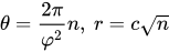
donde n es el índice de la flor y c es un factor de escala constante; las flores se encuentran así en la espiral de Fermat . El ángulo de divergencia , aproximadamente 137,51°, es el ángulo áureo , que divide el círculo en la proporción áurea. Debido a que esta proporción es irracional, ninguna flor tiene un vecino exactamente al mismo ángulo del centro, por lo que las flores se empaquetan de manera eficiente. Debido a que las aproximaciones racionales a la proporción áurea son de la forma F ( j ): F ( j +1) , los vecinos más cercanos de la flor número n son aquellos en n ± F ( j ) para algún índice j , que depende de r , la distancia desde el centro. Los girasoles y flores similares suelen tener espirales de flores en sentido horario y antihorario en la cantidad de números de Fibonacci adyacentes, [ 91 ] típicamente contados por el rango más externo de radios. [ 92 ]
Los números de Fibonacci también aparecen en los pedigríes ancestrales de las abejas (que son haplodiploides ), según las siguientes reglas:
- Si se pone un huevo pero no se fertiliza, nacerá un macho (o zángano en el caso de las abejas melíferas).
- Sin embargo, si un óvulo es fertilizado, produce una hembra.
Así, una abeja macho siempre tiene un progenitor, y una abeja hembra tiene dos. Si se rastrea el pedigrí de cualquier abeja macho (1 abeja), tiene 1 progenitor (1 abeja), 2 abuelos, 3 bisabuelos, 5 tatarabuelos, y así sucesivamente. Esta secuencia de números de progenitores es la secuencia de Fibonacci. El número de ancestros en cada nivel, F n , es el número de ancestros femeninos, que es F n −1 , más el número de ancestros masculinos, que es F n −2 . [ 93 ] [ 94 ] Esto se basa en la suposición poco realista de que los ancestros en cada nivel no están relacionados entre sí.

It has similarly been noticed that the number of possible ancestors on the human X chromosome inheritance line at a given ancestral generation also follows the Fibonacci sequence.[95] A male individual has an X chromosome, which he received from his mother, and a Y chromosome, which he received from his father. The male counts as the "origin" of his own X chromosome (), and at his parents' generation, his X chromosome came from a single parent (). The male's mother received one X chromosome from her mother (the son's maternal grandmother), and one from her father (the son's maternal grandfather), so two grandparents contributed to the male descendant's X chromosome (). The maternal grandfather received his X chromosome from his mother, and the maternal grandmother received X chromosomes from both of her parents, so three great-grandparents contributed to the male descendant's X chromosome (). Five great-great-grandparents contributed to the male descendant's X chromosome (), etc. (This assumes that all ancestors of a given descendant are independent, but if any genealogy is traced far enough back in time, ancestors begin to appear on multiple lines of the genealogy, until eventually a population founder appears on all lines of the genealogy.)


Other
- In optics, when a beam of light shines at an angle through two stacked transparent plates of different materials of different refractive indexes, it may reflect off three surfaces: the top, middle, and bottom surfaces of the two plates. The number of different beam paths that have k reflections, for k > 1, is the k-th Fibonacci number. (However, when k = 1, there are three reflection paths, not two, one for each of the three surfaces.)[96]
- Fibonacci retracement levels are widely used in technical analysis for financial market trading.
- Since the conversion factor 1.609344 for miles to kilometers is close to the golden ratio, the decomposition of distance in miles into a sum of Fibonacci numbers becomes nearly the kilometer sum when the Fibonacci numbers are replaced by their successors. This method amounts to a radix 2 number register in golden ratio baseφ being shifted. To convert from kilometers to miles, shift the register down the Fibonacci sequence instead.[97]
- Los valores medidos de voltajes y corrientes en el circuito de cadena de resistencias infinita (también llamado escalera de resistencias o circuito serie-paralelo infinito) siguen la secuencia de Fibonacci. Los resultados intermedios de la suma de las resistencias alternas en serie y en paralelo producen fracciones compuestas por números de Fibonacci consecutivos. La resistencia equivalente de todo el circuito es igual a la proporción áurea. [ 98 ]
- Brasch et al. (2012) muestran cómo una secuencia de Fibonacci generalizada también puede vincularse al campo de la economía . [ 99 ] En particular, se muestra cómo una secuencia de Fibonacci generalizada se incorpora a la función de control de problemas de optimización dinámica de horizonte finito con un estado y una variable de control. El procedimiento se ilustra con un ejemplo conocido como el modelo de crecimiento económico de Brock-Mirman.
- Mario Merz incluyó la secuencia de Fibonacci en algunas de sus obras de arte a partir de 1970. [ 100 ]
- Joseph Schillinger (1895–1943) desarrolló un sistema de composición que utiliza intervalos de Fibonacci en algunas de sus melodías; consideraba que estos eran el equivalente musical de la elaborada armonía evidente en la naturaleza. [ 101 ] Véase también Proporción áurea § Música .
- En el desarrollo de software , los números de Fibonacci son utilizados frecuentemente por equipos ágiles que operan bajo el marco Scrum para dimensionar los elementos de su backlog de producto . [ 102 ]
Véase también
- La Asociación Fibonacci – Organización para la investigación sobre los números de Fibonacci
- Los números de Fibonacci en la cultura popular
- Palabra de Fibonacci : secuencia binaria de la recurrencia de Fibonacci.
- Secuencia de Fibonacci aleatoria : secuencia matemática aleatoria basada en la secuencia de Fibonacci.
- Matriz de Wythoff : matriz infinita de números enteros derivada de la secuencia de Fibonacci.
- Conferencia Internacional sobre los Números de Fibonacci y sus Aplicaciones – Conferencia de Matemáticas
Referencias
Notas a pie de página explicativas
- ↑ "Para cuatro, al mezclarse variaciones de metros de dos [y] tres, se obtiene cinco. Para cinco, al mezclarse variaciones de dos anteriores, tres [y] cuatro, se obtiene ocho. De esta manera, para seis, al mezclarse [variaciones] de cuatro [y] de cinco, se obtiene trece. Y así, al mezclarse variaciones de dos metros anteriores, siete moras [son] veintiuna. De esta forma, el proceso debe seguirse en todos los mātrā-vṛttas" [ 14 ]
- ↑ Esto considera las operaciones aritméticas de precisión arbitraria como O (1) . Si se tiene en cuenta la longitud de bits, la exponenciación por cuadrado sigue siendo una mejora notable, pero la complejidad general está dominada por el último paso de multiplicación; hay O ( n ) dígitos en el resultado, y la tarea requiere producirlos todos.
Citas
- ↑ Richard A. Brualdi, Combinatoria introductoria , Quinta edición, Pearson, 2005
- ↑ Peter Cameron, Combinatoria: Temas, técnicas, algoritmos , Cambridge University Press, 1994
- 1 2 3 Goonatilake, Susantha (1998), Hacia una ciencia global , Indiana University Press, pág. 126, ISBN 978-0-253-33388-9
- 1 2 3 Singh, Parmanand (1985), "Los llamados números de Fibonacci en la India antigua y medieval", Historia Mathematica , 12 (3): 229– 244, doi : 10.1016/0315-0860(85)90021-7
- 1 2 Knuth, Donald (2006), El arte de la programación informática , vol. 4. Generación de todos los árboles: historia de la generación combinatoria, Addison–Wesley, pág. 50, ISBN 978-0-321-33570-8Era
natural considerar el conjunto de todas las secuencias de [L] y [S] que tienen exactamente m pulsos. ... hay exactamente Fm+1 de ellas. Por ejemplo, las 21 secuencias cuando m = 7 son: [da lista]. De esta manera, los prosodistas indios fueron llevados a descubrir la secuencia de Fibonacci, como hemos observado en la Sección 1.2.8 (desde v.1).
- ↑ Sigler 2002 , págs. 404–05.
- ↑ Lucas 1891 , pág. 3.
- ↑ Beck y Geoghegan 2010 .
- ↑ Bóna 2011 , pág. 180.
- ↑ Vajda, Steven (1989). Números de Fibonacci y Lucas, y la sección áurea: teoría y aplicaciones . Chichester: Ellis Horwood. pág. 10. ISBN 0-7458-0715-1.
- ↑ Knuth, Donald (1968), El arte de la programación informática , vol. 1, Addison Wesley, pág. 100, ISBN 978-81-7758-754-8Antes de
que Fibonacci escribiera su obra, la secuencia Fn ya había sido discutida por eruditos indios, quienes llevaban mucho tiempo interesados en los patrones rítmicos ... tanto Gopala (antes del 1135 d. C.) como Hemachandra (c. 1150) mencionaron explícitamente los números 1, 2, 3, 5, 8, 13, 21 [véase P. Singh Historia Math 12 (1985) 229–44]" pág. 100 (3.ª ed.) ...
- 1 2 Livio 2003 , pág. 197.
- ↑ Agrawala, VS (1969),Pāṇinikālīna Bhāratavarṣa (Hn.). Varanasi-I: TheChowkhamba Vidyabhawan ,
SadgurushiShya escribe que Pingala era un hermano menor de Pāṇini [Agrawala 1969, lb]. Existe una opinión alternativa que afirma que era un tío materno de Pāṇini [Vinayasagar 1965, Prefacio, 121]. ... Agrawala [1969, 463–76], tras una cuidadosa investigación en la que consideró las opiniones de estudiosos anteriores, concluyó que Pāṇini vivió entre el 480 y el 410 a. C.
- ↑ Velankar, HD (1962),'Vṛttajātisamuccaya' de kavi Virahanka , Jodhpur: Instituto de Investigaciones Orientales de Rajasthan, p. 101
- ^ Livio 2003 , págs. 197-198.
- ↑ Shah, Jayant (1991), A History of Piṅgala's Combinatorics (PDF) , Northeastern University , p. 41 , consultado el 4 de enero de 2019.
- ↑ Sigler 2002 , págs. 404–405.
- ↑ "Libro Abaci de Fibonacci (Libro de Cálculo)" , Universidad de Utah , 13 de diciembre de 2009 , consultado el 28 de noviembre de 2018.
- ↑ Tassone, Ann Dominic (abril de 1967), "Un par de conejos y un matemático", The Arithmetic Teacher , 14 (4): 285–288 , doi : 10.5951/at.14.4.0285 , JSTOR 41187298
- ↑ Knott, Ron, Los conejos de Fibonacci , Facultad de Ingeniería y Ciencias Físicas de la Universidad de Surrey
- ↑ Gardner, Martin (1996), Mathematical Circus , The Mathematical Association of America, p. 153, ISBN 978-0-88385-506-5
Resulta irónico que Leonardo, quien realizó valiosas contribuciones a las matemáticas, sea recordado hoy principalmente porque un teórico de números francés del siglo XIX, Édouard Lucas, le atribuyó el nombre de Fibonacci a una secuencia numérica que aparece en un problema trivial del Liber abaci
. - ↑ belcastro, sarah-marie (2018). Matemáticas discretas con patos (2.ª ed.). CRC Press. pág. 260. ISBN 978-1-351-68369-2.Extracto de la página 260
- ↑ Beutelspacher, Albrecht; Petri, Bernhard (1996), "Fibonacci-Zahlen", Der Goldene Schnitt , Einblick in die Wissenschaft, Vieweg+Teubner Verlag, págs. 87–98 , doi : 10.1007/978-3-322-85165-9_6 , ISBN 978-3-8154-2511-4
- ↑ Ball 2003 , pág. 156.
- ↑Ball 2003, pp. 155–156.
- ↑Sloane, N. J. A. (ed.), "SequenceA002390(Decimal expansion of natural logarithm of golden ratio)", The On-Line Encyclopedia of Integer Sequences, OEIS Foundation
- ↑Sloane, N. J. A. (ed.), "SequenceA097348(Decimal expansion of arccsch(2)/log(10))", The On-Line Encyclopedia of Integer Sequences, OEIS Foundation
- ↑Kepler, Johannes (1966), A New Year Gift: On Hexagonal Snow, Oxford University Press, p. 92, ISBN 978-0-19-858120-8
- ↑Strena seu de Nive Sexangula, 1611
- ↑Gessel, Ira (October 1972), "Fibonacci is a Square"(PDF), The Fibonacci Quarterly, 10 (4): 417–19, retrieved 2012-04-11
- ↑"The Golden Ratio, Fibonacci Numbers and Continued Fractions". nrich.maths.org. Retrieved 2024-03-22.
- ↑Dijkstra, Edsger W. (1978), In honour of Fibonacci(PDF)
- ↑Lucas 1891, p. 4.
- ↑Vorobiev, Nikolaĭ Nikolaevich; Martin, Mircea (2002), "Chapter 1", Fibonacci Numbers, Birkhäuser, pp. 5–6, ISBN 978-3-7643-6135-8
- 123Weisstein, Eric W., "Fibonacci Number", MathWorld
- ↑Glaister, P (1995), "Fibonacci power series", The Mathematical Gazette, 79 (486): 521–25, doi:10.2307/3618079, JSTOR 3618079, S2CID 116536130
- ↑Landau, Edmund (1899), "Sur la Série des Invers de Nombres de Fibonacci" [On the Series of Inverse Fibonacci Numbers], Bull. Soc. Math. France (in French), 27: 298–300, quoted accordingly in Borwein & Borwein (1998), p. 95, exercise 3b.
- ↑Sloane, N. J. A. (ed.), "SequenceA079586(Decimal expansion of Sum_{k>=1} 1/F(k) where F(k) is the k-th Fibonacci number)", The On-Line Encyclopedia of Integer Sequences, OEIS Foundation
- ↑André-Jeannin, Richard (1989), "Irrationalité de la somme des inverses de certaines suites récurrentes" [Irrationality of the sum of the reciprocals of certain recurrence sequences], Comptes Rendus de l'Académie des Sciences Série I Sciences mathématiques (in French), 308 (19): 539–41, MR 0999451
- ↑Honsberger 1985, pp. 135–136.
- ↑Ribenboim, Paulo (2000), My Numbers, My Friends, Springer-Verlag
- ↑Su, Francis E. (2000), "Fibonacci GCD's, Please", Mudd Math Fun Facts, Harvey Mudd College Math Department, archived from the original on 2009-12-14, retrieved 2007-02-23
- ↑Williams, H. C. (1982), "A note on the Fibonacci quotient ", Canadian Mathematical Bulletin, 25 (3): 366–70, doi:10.4153/CMB-1982-053-0, hdl:10338.dmlcz/137492, MR 0668957. Williams calls this property "well known".
- ↑Prime Numbers, Richard Crandall, Carl Pomerance, Springer, second edition, 2005, p. 142.
- ↑Sloane, N. J. A. (ed.), "SequenceA005478(Prime Fibonacci numbers)", The On-Line Encyclopedia of Integer Sequences, OEIS Foundation
- ↑Diaconis, Persi (2018), "Probabilizing Fibonacci numbers"(PDF), in Butler, Steve; Cooper, Joshua; Hurlbert, Glenn (eds.), Connections in Discrete Mathematics: A Celebration of the Work of Ron Graham, Cambridge University Press, pp. 1–12, ISBN 978-1-107-15398-1, MR 3821829, archived from the original(PDF) on 2023-11-18, retrieved 2022-11-23
- ↑Honsberger 1985, p. 133.
- ↑ Cohn, JHE (1964), "Sobre los números de Fibonacci cuadrados", The Journal of the London Mathematical Society , 39 : 537–540 , doi : 10.1112/jlms/s1-39.1.537 , MR 0163867
- ^ Pethő, Attila (2001), "Propiedades diofánticas de secuencias recursivas lineales II", Acta Mathematica Academiae Paedagogicae Nyíregyháziensis , 17 : 81– 96
- ↑ Bugeaud, Y; Mignotte, M; Siksek, S (2006), "Enfoques clásicos y modulares para ecuaciones diofánticas exponenciales. I. Potencias perfectas de Fibonacci y Lucas", Ann. Math. , 2 (163): 969– 1018, arXiv : math/0403046 , Bibcode : 2004math......3046B , doi : 10.4007/annals.2006.163.969 , S2CID 10266596
- ↑ Luo, Ming (1989), "Sobre los números triangulares de Fibonacci" (PDF) , Fibonacci Quart. , 27 (2): 98–108 , doi : 10.1080/00150517.1989.12429576
- ^ Luca, Florian (2000), "Números perfectos de Fibonacci y Lucas", Rediconti del Circolo Matematico di Palermo , 49 (2): 313– 18, doi : 10.1007/BF02904236 , ISSN 1973-4409 , MR 1765401 , S2CID 121789033
- ↑ Broughan, Kevin A.; González, Marcos J.; Lewis, Ryan H.; Luca, Florian; Mejía Huguet, V. Janitzio; Togbé, Alain (2011), "No existen números de Fibonacci multiplicativamente perfectos" , Integers , 11a : A7, MR 2988067
- ↑ Luca, Florian; Mejía Huguet, V. Janitzio (2010), "Sobre los números perfectos que son razones de dos números de Fibonacci" , Annales Mathematicae at Informaticae , 37 : 107–24 , ISSN 1787-6117 , MR 2753031
- ↑ Knott, Ron, Los números de Fibonacci , Reino Unido: Surrey
- ↑ Sloane, N. J. A. (ed.), "Secuencia A235383 (números de Fibonacci que son producto de otros números de Fibonacci)" , La enciclopedia en línea de secuencias de enteros , Fundación OEIS
- ↑ Ribenboim, Paulo (1996), El nuevo libro de registros de números primos , Nueva York: Springer, pág. 64, ISBN 978-0-387-94457-9
- ↑ Lemmermeyer 2000 , págs. 73–74, ej. 2.25–28.
- ↑ Lemmermeyer 2000 , págs. 73–74, ej. 2.28.
- ↑ Lemmermeyer 2000 , pág. 73, ej. 2.27.
- ↑ Factorizaciones de Fibonacci y Lucas , MersennusRecopila todos los factores conocidos de F ( i ) con i < 10000
- ↑ Factores de los números de Fibonacci y Lucas , Rojo golpeRecopila todos los factores conocidos de F ( i ) con 10000 < i < 50000
- ↑ Freyd, Peter; Brown, Kevin S. (1993), "Problemas y soluciones: Soluciones: E3410", The American Mathematical Monthly , 99 (3): 278–79 , doi : 10.2307/2325076 , JSTOR 2325076
- ↑ Sloane, N. J. A. (ed.), "Secuencia A001175 (períodos de Pisano (o números de Pisano): período de números de Fibonacci módulo n)" , La enciclopedia en línea de secuencias de enteros , Fundación OEIS
- ↑ Lü, Kebo; Wang, Jun (2006), " k -step Fibonacci sequence módulo m " , Utilitas Mathematica , 71 : 169– 177, MR 2278830
- ↑ Hoggatt Jr, VE; Bicknell, Marjorie (1973), "Polinomios de Fibonacci generalizados", The Fibonacci Quarterly , 11 (5), Taylor & Francis
- ↑ Lucas 1891 , pág. 7.
- ↑ Stanley, Richard (2011), Combinatoria enumerativa I (2.ª ed.) , Cambridge Univ. Press, pág. 121, ej. 1.35, ISBN 978-1-107-60262-5
- ^ Harizanov, Valentina (1995), "Revisión de Yuri V. Matiyasevich, El décimo problema de Hibert " , Modern Logic , 5 (3): 345– 55
- ↑ Pagni, David (septiembre de 2001), "Fibonacci se encuentra con Pitágoras", Matemáticas en la escuela , 30 (4): 39– 40, JSTOR 30215477
- ↑ Stephenson, Kenneth (2005), Introducción al empaquetamiento de círculos: La teoría de las funciones analíticas discretas , Cambridge University Press, ISBN 978-0-521-82356-2, MR 2131318 ; véase especialmente el Lema 8.2 (Lema del Anillo), págs. 73–74 , y el Apéndice B, El Lema del Anillo, págs. 318–321.
- ↑ Knuth, Donald E (1997), El arte de la programación informática , vol. 1: Algoritmos fundamentales (3.ª ed.), Addison–Wesley, pág. 343, ISBN 978-0-201-89683-1
- ↑ Adelson-Velsky, Georgy; Landis, Evgenii ( 1962), "Un algoritmo para la organización de la información", Actas de la Academia de Ciencias de la URSS (en ruso), 146 : 263–266Traducción al inglés de Myron J. Ricci en Soviet Mathematics - Doklady , 3:1259–1263, 1962.
- ↑ Avriel, M; Wilde, DJ (1966), "Optimalidad de la técnica de búsqueda simétrica de Fibonacci", Fibonacci Quarterly (3): 265– 69, doi : 10.1080/00150517.1966.12431364
- ↑ Manual de referencia del núcleo ROM de Amiga , Addison–Wesley, 1991
- ↑ "IFF", Wiki multimedia
- ↑ Dean Leffingwell (1 de julio de 2021), Historia , Marco de trabajo ágil escalado , consultado el 15 de agosto de 2022
- ↑ Nayak, Chetan; Simon, Steven H.; Stern, Ady; Freedman, Michael; Das Sarma, Sankar (2008-09-12). "Aniones no abelianos y computación cuántica topológica" . Reviews of Modern Physics . 80 (3): 1083– 1159. arXiv : 0707.1889 . doi : 10.1103/RevModPhys.80.1083 .
- ↑ Simon, Steven H. (29 de septiembre de 2023). Topological Quantum . Oxford University Press. Oxford. pág. 98. doi : 10.1093/oso/9780198886723.001.0001 . ISBN 0-19-888672-1.
- ↑ Douady, S; Couder, Y (1996), "Filotaxis como un proceso dinámico de autoorganización" (PDF) , Journal of Theoretical Biology , 178 (3): 255–74 , doi : 10.1006/jtbi.1996.0026 , archivado del original (PDF) el 26 de mayo de 2006
- ↑ Jones, Judy; Wilson, William (2006), "Ciencia", Una educación incompleta , Ballantine Books, pág. 544, ISBN 978-0-7394-7582-9
- ↑"The Wonder of Fibonacci in our Gardens | UC Master Gardeners of San Mateo & San Francisco Counties". ucanr.edu. Retrieved 2025-11-18.
- ↑Brousseau, A (1969), "Fibonacci Statistics in Conifers", Fibonacci Quarterly, 7 (5): 525–32, doi:10.1080/00150517.1969.12431136
- ↑"Marks for the da Vinci Code: B–", Maths, Computer Science For Fun: CS4FN
- ↑Scott, T.C.; Marketos, P. (March 2014), On the Origin of the Fibonacci Sequence(PDF), MacTutor History of Mathematics archive, University of St Andrews
- ↑Livio 2003, p. 110.
- ↑Livio 2003, pp. 112–13.
- ↑Varenne, Franck (2010), Formaliser le vivant - Lois, Théories, Modèles (in French), Hermann, p. 28, ISBN 9782705678128, retrieved 2022-10-30,
En 1830, K. F. Schimper et A. Braun [...]. Ils montraient que si l'on représente cet angle de divergence par une fraction reflétant le nombre de tours par feuille ([...]), on tombe régulièrement sur un des nombres de la suite de Fibonacci pour le numérateur [...].
- ↑Prusinkiewicz, Przemyslaw; Hanan, James (1989), Lindenmayer Systems, Fractals, and Plants (Lecture Notes in Biomathematics), Springer-Verlag, ISBN 978-0-387-97092-9
- ↑Vogel, Helmut (1979), "A better way to construct the sunflower head", Mathematical Biosciences, 44 (3–4): 179–89, doi:10.1016/0025-5564(79)90080-4
- ↑Livio 2003, p. 112.
- ↑Prusinkiewicz, Przemyslaw; Lindenmayer, Aristid (1990), "4", The Algorithmic Beauty of Plants, Springer-Verlag, pp. 101–107, ISBN 978-0-387-97297-8
- ↑Basin, S. L. (1963), "The Fibonacci sequence as it appears in nature"(PDF), The Fibonacci Quarterly, 1 (1): 53–56, doi:10.1080/00150517.1963.12431602
- ↑Yanega, D. 1996. Sex ratio and sex allocation in sweat bees (Hymenoptera: Halictidae). J. Kans. Ent. Soc. 69 Suppl.: 98-115.
- 12Hutchison, Luke (September 2004), "Growing the Family Tree: The Power of DNA in Reconstructing Family Relationships"(PDF), Proceedings of the First Symposium on Bioinformatics and Biotechnology (BIOT-04), archived from the original(PDF) on 2020-09-25, retrieved 2016-09-03
- ↑Livio 2003, pp. 98–99.
- ↑"Zeckendorf representation", Encyclopedia of Math
- ↑Patranabis, D.; Dana, S. K. (December 1985), "Single-shunt fault diagnosis through terminal attenuation measurement and using Fibonacci numbers", IEEE Transactions on Instrumentation and Measurement, IM-34 (4): 650–653, Bibcode:1985ITIM...34..650P, doi:10.1109/tim.1985.4315428, S2CID 35413237
- ↑Brasch, T. von; Byström, J.; Lystad, L.P. (2012), "Optimal Control and the Fibonacci Sequence", Journal of Optimization Theory and Applications, 154 (3): 857–78, doi:10.1007/s10957-012-0061-2, hdl:11250/180781, S2CID 8550726
- ↑Livio 2003, p. 176.
- ↑Livio 2003, p. 193.
- ↑Kathuria, Madhur. "A Guide to Using the Fibonacci Sequence in Scrum". Scrum Alliance. Retrieved 8 August 2025.

Works cited
- Ball, Keith M (2003), "8: Fibonacci's Rabbits Revisited", Strange Curves, Counting Rabbits, and Other Mathematical Explorations, Princeton, NJ: Princeton University Press, ISBN 978-0-691-11321-0.
- Beck, Matthias; Geoghegan, Ross (2010), The Art of Proof: Basic Training for Deeper Mathematics, New York: Springer, ISBN 978-1-4419-7022-0.
- Bóna, Miklós (2011), A Walk Through Combinatorics (3rd ed.), New Jersey: World Scientific, ISBN 978-981-4335-23-2.
- Borwein, Jonathan M.; Borwein, Peter B. (July 1998), Pi and the AGM: A Study in Analytic Number Theory and Computational Complexity, Wiley, pp. 91–101, ISBN 978-0-471-31515-5
- Honsberger, Ross (1985), "Una segunda mirada a los números de Fibonacci y Lucas", Mathematical Gems III , Dolciani Mathematical Expositions, vol. 9, American Mathematical Society, pp. 102–138 , ISBN 9781470457181
- Lemmermeyer, Franz (2000), Leyes de reciprocidad: De Euler a Eisenstein , Monografías de Springer en matemáticas, Nueva York: Springer, ISBN 978-3-540-66957-9.
- Livio, Mario (2003) [2002], La proporción áurea: La historia de Phi, el número más asombroso del mundo (Primera edición en rústica ), Nueva York: Broadway Books , ISBN 0-7679-0816-3
- Lucas, Édouard (1891), Théorie des nombres (en francés), vol. 1, París: Gauthier-Villars.
- Sigler, LE (2002), El Liber Abaci de Fibonacci: una traducción al inglés moderno del Libro de Cálculo de Leonardo Pisano , Fuentes y estudios en la historia de las matemáticas y las ciencias físicas, Springer, ISBN 978-0-387-95419-6
Enlaces externos
- Secuencia de Fibonacci y proporción áurea: Las matemáticas en el mundo moderno - Mathuklasan con Sir Ram en YouTube - animación de secuencia, espiral, proporción áurea, crecimiento de pares de conejos. Ejemplos en arte, música, arquitectura, naturaleza y astronomía.
- Períodos de secuencias de Fibonacci (Mod m) en MathPages
- Los científicos encuentran pistas sobre la formación de espirales de Fibonacci en la naturaleza.
- La secuencia de Fibonacci en el programa "In Our Time " de la BBC.
- "Números de Fibonacci" , Enciclopedia de Matemáticas , EMS Press , 2001 [1994]
- Números de Fibonacci
- Secuencias de enteros




