 Hispanopedia Wiki
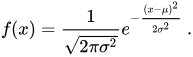
En teoría de probabilidad y estadística , una distribución normal o distribución gaussiana es un tipo de distribución de probabilidad continua para una variable aleatoria de valor real . La forma general de su función de densidad de probabilidad es El parámetro es la media o esperanza de la distribución (y también su mediana y moda ), mientras que el parámetro es la varianza . La desviación estándar de la distribución es (sigma). Se dice que una variable aleatoria con una distribución gaussiana tiene una distribución normal y se denomina desviación normal .


Las distribuciones normales son importantes en estadística y se utilizan a menudo en las ciencias naturales y sociales para representar variables aleatorias de valor real cuyas distribuciones no se conocen. [2] [3] Su importancia se debe en parte al teorema del límite central . Este afirma que, en determinadas condiciones, el promedio de muchas muestras (observaciones) de una variable aleatoria con media y varianza finitas es en sí mismo una variable aleatoria, cuya distribución converge a una distribución normal a medida que aumenta el número de muestras. Por lo tanto, las cantidades físicas que se espera que sean la suma de muchos procesos independientes, como los errores de medición , a menudo tienen distribuciones que son casi normales. [4]
Además, las distribuciones gaussianas tienen algunas propiedades únicas que son valiosas en los estudios analíticos. Por ejemplo, cualquier combinación lineal de un conjunto fijo de desviaciones normales independientes es una desviación normal. Muchos resultados y métodos, como la propagación de la incertidumbre y el ajuste de parámetros por mínimos cuadrados [5] , se pueden derivar analíticamente en forma explícita cuando las variables relevantes se distribuyen normalmente.
A veces, a una distribución normal se la denomina informalmente curva de campana . [6] Sin embargo, muchas otras distribuciones tienen forma de campana (como la distribución de Cauchy , la t de Student y las distribuciones logísticas ). Para conocer otros nombres, consulte Nomenclatura .
La distribución de probabilidad univariante se generaliza para vectores en la distribución normal multivariante y para matrices en la distribución normal matricial .
Definiciones
Distribución normal estándar
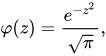
El caso más simple de una distribución normal se conoce como distribución normal estándar o distribución normal unitaria . Este es un caso especial cuando y , y se describe mediante esta función de densidad de probabilidad (o densidad): La variable tiene una media de 0 y una varianza y desviación estándar de 1. La densidad tiene su pico en y puntos de inflexión en y .


Aunque la densidad anterior se conoce más comúnmente como la normal estándar, algunos autores han utilizado ese término para describir otras versiones de la distribución normal. Carl Friedrich Gauss , por ejemplo, una vez definió la normal estándar como que tiene una varianza de , y Stephen Stigler [7] una vez definió la normal estándar como que tiene una forma funcional simple y una varianza de


Distribución normal general
Toda distribución normal es una versión de la distribución normal estándar, cuyo dominio ha sido ampliado por un factor (la desviación estándar) y luego traducido por (el valor medio):

La densidad de probabilidad debe escalarse de modo que la integral siga siendo 1.

Si es una desviación normal estándar , entonces tendrá una distribución normal con valor esperado y desviación estándar . Esto es equivalente a decir que la distribución normal estándar se puede escalar/estirar por un factor de y desplazar por para producir una distribución normal diferente, llamada . Por el contrario, si es una desviación normal con parámetros y , entonces esta distribución se puede volver a escalar y desplazar mediante la fórmula para convertirla en la distribución normal estándar. Esta variante también se denomina forma estandarizada de .



Notación
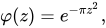
La densidad de probabilidad de la distribución gaussiana estándar (distribución normal estándar, con media cero y varianza unitaria) se denota a menudo con la letra griega ( phi ). [8] La forma alternativa de la letra griega phi, , también se utiliza con bastante frecuencia.


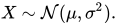
La distribución normal a menudo se denomina o . [9] Por lo tanto, cuando una variable aleatoria se distribuye normalmente con media y desviación estándar , se puede escribir


Parametrizaciones alternativas
Algunos autores abogan por utilizar la precisión como parámetro que define el ancho de la distribución, en lugar de la desviación estándar o la varianza . La precisión se define normalmente como el recíproco de la varianza, . [10] La fórmula para la distribución se convierte entonces en


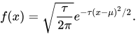
Se afirma que esta elección tiene ventajas en los cálculos numéricos cuando está muy cerca de cero y simplifica las fórmulas en algunos contextos, como en la inferencia bayesiana de variables con distribución normal multivariada .
Alternativamente, el recíproco de la desviación estándar podría definirse como la precisión , en cuyo caso la expresión de la distribución normal se convierte en


Según Stigler, esta formulación es ventajosa debido a una fórmula mucho más simple y fácil de recordar, y a fórmulas aproximadas simples para los cuantiles de la distribución.
Las distribuciones normales forman una familia exponencial con parámetros naturales y , y estadísticas naturales x y x 2 . Los parámetros de expectativa dual para la distribución normal son η 1 = μ y η 2 = μ 2 + σ 2 .


Función de distribución acumulativa
La función de distribución acumulativa (CDF) de la distribución normal estándar, usualmente denotada con la letra griega mayúscula ( phi ), es la integral


Función de error
La función de error relacionada da la probabilidad de una variable aleatoria, con distribución normal de media 0 y varianza 1/2 dentro del rango . Es decir:

![{\textstyle [-x,x]}](https://wikimedia.org/api/rest_v1/media/math/render/svg/4939f2eb7c55ff4e7d13331fc0599a5f2452b479)

Estas integrales no se pueden expresar en términos de funciones elementales y, a menudo, se dice que son funciones especiales . Sin embargo, se conocen muchas aproximaciones numéricas; consulte más información a continuación.
Las dos funciones están estrechamente relacionadas, a saber:
![{\displaystyle \Phi (x)={\frac {1}{2}}\left[1+\operatorname {erf} \left({\frac {x}{\sqrt {2}}}\right)\right]\,.}](https://wikimedia.org/api/rest_v1/media/math/render/svg/4dec6de19ebeaa734086622f167d87ac41e7b50d)
Para una distribución normal genérica con densidad , media y varianza , la función de distribución acumulativa es

![{\displaystyle F(x)=\Phi \left({\frac {x-\mu }{\sigma }}\right)={\frac {1}{2}}\left[1+\operatorname {erf} \left({\frac {x-\mu }{\sigma {\sqrt {2}}}}\right)\right]\,.}](https://wikimedia.org/api/rest_v1/media/math/render/svg/f48cf2d3b65754e434e6a6c5a90908dd83d44f12)
El complemento de la función de distribución acumulativa normal estándar, , se suele denominar función Q , especialmente en textos de ingeniería. [11] [12] Da la probabilidad de que el valor de una variable aleatoria normal estándar supere a : . Otras definiciones de la función -, todas las cuales son transformaciones simples de , también se utilizan ocasionalmente. [13]


La gráfica de la función de distribución acumulativa normal estándar tiene simetría rotacional doble alrededor del punto (0,1/2); es decir, . Su antiderivada (integral indefinida) se puede expresar de la siguiente manera:


La función de distribución acumulativa de la distribución normal estándar se puede ampliar mediante la integración por partes en una serie:
![{\displaystyle \Phi(x)={\frac {1}{2}}+{\frac {1}{\sqrt {2\pi }}}\cdot e^{-x^{2}/2}\left[x+{\frac {x^{3}}{3}}+{\frac {x^{5}}{3\cdot 5}}+\cdots +{\frac {x^{2n+1}}{(2n+1)!!}}+\cdots \right]\,.}](https://wikimedia.org/api/rest_v1/media/math/render/svg/ad8275ec6180f68c2dae03c9e70716b75ff4f3aa)
donde denota el factorial doble .

También se puede derivar una expansión asintótica de la función de distribución acumulativa para valores grandes de x mediante la integración por partes. Para obtener más información, consulte Función de error#Expansión asintótica . [14]
Se puede encontrar una aproximación rápida a la función de distribución acumulativa de la distribución normal estándar utilizando una aproximación de la serie de Taylor:

Cálculo recursivo con desarrollo de la serie de Taylor
La naturaleza recursiva de la familia de derivadas se puede utilizar para construir fácilmente una expansión de la serie de Taylor rápidamente convergente utilizando entradas recursivas sobre cualquier punto de valor conocido de la distribución :


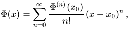
dónde:

Utilizando la serie de Taylor y el método de Newton para la función inversa
Una aplicación de la expansión de la serie de Taylor anterior es utilizar el método de Newton para invertir el cálculo. Es decir, si tenemos un valor para la función de distribución acumulativa , , pero no conocemos la x necesaria para obtener , podemos utilizar el método de Newton para encontrar x, y utilizar la expansión de la serie de Taylor anterior para minimizar el número de cálculos. El método de Newton es ideal para resolver este problema porque la primera derivada de , que es una integral de la distribución estándar normal, es la distribución estándar normal y está disponible para su uso en la solución del método de Newton.

Para resolver, seleccione una solución aproximada conocida, , para el . deseado puede ser un valor de una tabla de distribución, o una estimación inteligente seguida de un cálculo de utilizando cualquier medio deseado para calcular. Utilice este valor de y la expansión de la serie de Taylor anterior para minimizar los cálculos.

Repita el siguiente proceso hasta que la diferencia entre el calculado y el deseado , que llamaremos , esté por debajo de un error aceptablemente pequeño, como 10 −5 , 10 −15 , etc.:


dónde
- es la solución de una serie de Taylor usando y


Cuando los cálculos repetidos convergen a un error inferior al valor aceptablemente pequeño elegido, x será el valor necesario para obtener a del valor deseado, .
Desviación estándar y cobertura

Alrededor del 68% de los valores extraídos de una distribución normal están dentro de una desviación estándar σ de la media; alrededor del 95% de los valores se encuentran dentro de dos desviaciones estándar; y alrededor del 99,7% están dentro de tres desviaciones estándar. [6] Este hecho se conoce como la regla 68-95-99,7 (empírica) o la regla de 3 sigma .
Más precisamente, la probabilidad de que una desviación normal se encuentre en el rango entre y está dada por Para 12 dígitos significativos, los valores para son:




Para valores grandes , se puede utilizar la aproximación .


Función cuantil
La función cuantil de una distribución es la inversa de la función de distribución acumulativa. La función cuantil de la distribución normal estándar se denomina función probit y se puede expresar en términos de la función de error inversa : Para una variable aleatoria normal con media y varianza , la función cuantil es El cuantil de la distribución normal estándar se denota comúnmente como . Estos valores se utilizan en pruebas de hipótesis , construcción de intervalos de confianza y gráficos Q-Q . Una variable aleatoria normal excederá con probabilidad , y quedará fuera del intervalo con probabilidad . En particular, el cuantil es 1,96 ; por lo tanto, una variable aleatoria normal quedará fuera del intervalo solo en el 5% de los casos.




La siguiente tabla muestra el cuartil que se encontrará en el rango con una probabilidad especificada . Estos valores son útiles para determinar el intervalo de tolerancia para promedios de muestra y otros estimadores estadísticos con distribuciones normales (o asintóticamente normales). [15] La siguiente tabla muestra , no como se definió anteriormente.


Para números pequeños , la función cuantil tiene la expansión asintótica útil [ cita requerida ]

Propiedades
La distribución normal es la única distribución cuyos cumulantes más allá de los dos primeros (es decir, distintos de la media y la varianza ) son cero. También es la distribución continua con la entropía máxima para una media y varianza especificadas. [16] [17] Geary ha demostrado, suponiendo que la media y la varianza son finitas, que la distribución normal es la única distribución donde la media y la varianza calculadas a partir de un conjunto de valores extraídos independientes son independientes entre sí. [18] [19]
La distribución normal es una subclase de las distribuciones elípticas . La distribución normal es simétrica respecto de su media y no es cero en toda la línea real. Como tal, puede no ser un modelo adecuado para variables que son inherentemente positivas o fuertemente sesgadas, como el peso de una persona o el precio de una acción . Dichas variables pueden describirse mejor mediante otras distribuciones, como la distribución log-normal o la distribución de Pareto .
El valor de la distribución normal es prácticamente cero cuando el valor se encuentra a más de unas pocas desviaciones estándar de la media (por ejemplo, una dispersión de tres desviaciones estándar cubre toda la distribución total, excepto el 0,27%). Por lo tanto, puede no ser un modelo apropiado cuando se espera una fracción significativa de valores atípicos (valores que se encuentran a muchas desviaciones estándar de la media) y los mínimos cuadrados y otros métodos de inferencia estadística que son óptimos para las variables distribuidas normalmente suelen volverse muy poco confiables cuando se aplican a esos datos. En esos casos, se debe suponer una distribución de colas más pesadas y aplicar los métodos de inferencia estadística robustos adecuados .
La distribución gaussiana pertenece a la familia de distribuciones estables que son las que atraen las sumas de distribuciones independientes idénticamente distribuidas, independientemente de que la media o la varianza sean finitas o no. A excepción de la gaussiana, que es un caso límite, todas las distribuciones estables tienen colas pesadas y varianza infinita. Es una de las pocas distribuciones que son estables y que tienen funciones de densidad de probabilidad que se pueden expresar analíticamente, las otras son la distribución de Cauchy y la distribución de Lévy .
Simetrías y derivadas
La distribución normal con densidad (media y varianza ) tiene las siguientes propiedades:


- Es simétrica alrededor del punto que es al mismo tiempo la moda , la mediana y la media de la distribución. [20]
- Es unimodal : su primera derivada es positiva para negativa para y cero sólo en
- El área delimitada por la curva y el eje es la unidad (es decir, igual a uno).
- Su primera derivada es
- Su segunda derivada es
- Su densidad tiene dos puntos de inflexión (donde la segunda derivada de es cero y cambia de signo), ubicados a una desviación estándar de la media, es decir en y [20]
- Su densidad es logarítmica-cóncava . [20]
- Su densidad es infinitamente diferenciable , de hecho supersuave , de orden 2. [21]


Además, la densidad de la distribución normal estándar (es decir, y ) también tiene las siguientes propiedades:

- Su primera derivada es
- Su segunda derivada es
- De manera más general, su derivada n- ésima es donde es el n -ésimo polinomio de Hermite (probabilista) . [22]
- La probabilidad de que una variable distribuida normalmente con y conocidos esté en un conjunto particular, se puede calcular utilizando el hecho de que la fracción tiene una distribución normal estándar.


Momentos
Los momentos simples y absolutos de una variable son los valores esperados de y , respectivamente. Si el valor esperado de es cero, estos parámetros se denominan momentos centrales; de lo contrario, estos parámetros se denominan momentos no centrales. Por lo general, solo nos interesan los momentos con orden entero .


Si tiene una distribución normal, los momentos no centrales existen y son finitos para cualquier número cuya parte real sea mayor que −1. Para cualquier entero no negativo , los momentos centrales simples son: [23] Aquí denota el factorial doble , es decir, el producto de todos los números de a 1 que tienen la misma paridad que
![{\displaystyle \operatorname {E} \left[(X-\mu )^{p}\right]={\begin{cases}0&{\text{si }}p{\text{ es impar,}}\\\sigma ^{p}(p-1)!!&{\text{si }}p{\text{ es par.}}\end{cases}}}](https://wikimedia.org/api/rest_v1/media/math/render/svg/f1d2c92b62ac2bbe07a8e475faac29c8cc5f7755)


Los momentos absolutos centrales coinciden con los momentos simples para todos los órdenes pares, pero son distintos de cero para los órdenes impares. Para cualquier entero no negativo

La última fórmula es válida también para cualquier número no entero. Cuando la media de los momentos simples y absolutos se pueden expresar en términos de funciones hipergeométricas confluentes y [24]
![{\displaystyle {\begin{aligned}\operatorname {E} \left[|X-\mu |^{p}\right]&=\sigma ^{p}(p-1)!!\cdot {\begin{cases}{\sqrt {\frac {2}{\pi }}}&{\text{si }}p{\text{ es impar}}\\1&{\text{si }}p{\text{ es par}}\end{cases}}\\&=\sigma ^{p}\cdot {\frac {2^{p/2}\Gamma \left({\frac {p+1}{2}}\right)}{\sqrt {\pi }}}.\end{aligned}}}](https://wikimedia.org/api/rest_v1/media/math/render/svg/3b196371c491676efa7ea7770ef56773db7652cd)


![{\displaystyle {\begin{aligned}\nombredeloperador {E} \left[X^{p}\right]&=\sigma ^{p}\cdot (-i{\sqrt {2}})^{p}U\left(-{\frac {p}{2}},{\frac {1}{2}},-{\frac {1}{2}}\left({\frac {\mu }{\sigma }}\right)^{2}\right),\\\nombredeloperador {E} \left[|X|^{p}\right]&=\sigma ^{p}\cdot 2^{p/2}{\frac {\Gamma \left({\frac {1+p}{2}}\right)}{\sqrt {\pi }}}{}_{1}F_{1}\left(-{\frac {p}{2}},{\frac {1}{2}},-{\frac {1}{2}}\left({\frac {\mu }{\sigma }}\right)^{2}\right).\end{alineado}}}](https://wikimedia.org/api/rest_v1/media/math/render/svg/0c17bf881593b86e728bf5dfbdb41a4b86da3875)
Estas expresiones siguen siendo válidas incluso si no es un número entero. Véase también polinomios de Hermite generalizados .
La esperanza de condicionada al evento que se encuentra en un intervalo está dada por donde y respectivamente son la densidad y la función de distribución acumulada de . Esto se conoce como el coeficiente de Mills inverso . Tenga en cuenta que anteriormente, se utiliza la densidad de en lugar de la densidad normal estándar como en el coeficiente de Mills inverso, por lo que aquí tenemos en lugar de .
![{\textstyle [a,b]}](https://wikimedia.org/api/rest_v1/media/math/render/svg/2c780cbaafb5b1d4a6912aa65d2b0b1982097108)
![{\displaystyle \operatorname {E} \left[X\mid a<X<b\right]=\mu -\sigma ^{2}{\frac {f(b)-f(a)}{F(b)-F(a)}}\,,}](https://wikimedia.org/api/rest_v1/media/math/render/svg/ad97cc40960e6d1d4e65f51596c9cd0c9accfdc0)


Transformada de Fourier y función característica
La transformada de Fourier de una densidad normal con media y varianza es [25]

donde es la unidad imaginaria . Si la media , el primer factor es 1, y la transformada de Fourier es, además de un factor constante, una densidad normal en el dominio de la frecuencia , con media 0 y varianza . En particular, la distribución normal estándar es una función propia de la transformada de Fourier.

En teoría de la probabilidad, la transformada de Fourier de la distribución de probabilidad de una variable aleatoria de valor real está estrechamente relacionada con la función característica de esa variable, que se define como el valor esperado de , en función de la variable real (el parámetro de frecuencia de la transformada de Fourier). Esta definición se puede extender analíticamente a una variable de valor complejo . [26] La relación entre ambas es:


Funciones generadoras de momentos y cumulantes
La función generadora de momentos de una variable aleatoria real es el valor esperado de , en función del parámetro real . Para una distribución normal con densidad , media y varianza , la función generadora de momentos existe y es igual a

Para cualquier , el coeficiente de en la función generadora de momentos (expresada como una serie de potencia exponencial en ) es el valor esperado de la distribución normal .
![{\displaystyle M(t)=\operatorname {E} \left[e^{tX}\right]={\hat {f}}(it)=e^{\mu t}e^{\sigma ^{2}t^{2}/2}\,.}](https://wikimedia.org/api/rest_v1/media/math/render/svg/3b5930b107fb4328bc04d077d65ce3d2bf1510de)


![{\displaystyle E[X^{k}]}](https://wikimedia.org/api/rest_v1/media/math/render/svg/4dcd54fe6c5cb4afbfcd7bd94c4778d13b8bbc3f)
La función generadora cumulante es el logaritmo de la función generadora de momentos, es decir

Los coeficientes de esta serie de potencias exponenciales definen los cumulantes, pero como se trata de un polinomio cuadrático en , solo los dos primeros cumulantes son distintos de cero, es decir, la media y la varianza .

Algunos autores prefieren trabajar con la función característica E[ e itX ] = e iμt − σ 2 t 2 /2 y ln E[ e itX ] = iμt − 1/2 σ2t2 .
Operador y clase Stein
Dentro del método de Stein, el operador de Stein y la clase de una variable aleatoria son y la clase de todas las funciones absolutamente continuas .


![{\textstyle f:\mathbb {R} \to \mathbb {R} {\mbox{ tal que }}\mathbb {E} [|f'(X)|]<\infty }](https://wikimedia.org/api/rest_v1/media/math/render/svg/533b737bedccd7496f904d18a4fd39fade40b282)
Límite de varianza cero
En el límite cuando tiende a cero, la densidad de probabilidad tiende eventualmente a cero en cualquier , pero crece sin límite si , mientras que su integral permanece igual a 1. Por lo tanto, la distribución normal no puede definirse como una función ordinaria cuando .


Sin embargo, se puede definir la distribución normal con varianza cero como una función generalizada ; específicamente, como una función delta de Dirac traducida por la media , es decir Su función de distribución acumulativa es entonces la función escalón de Heaviside traducida por la media , es decir


Entropía máxima
De todas las distribuciones de probabilidad sobre los números reales con una media finita especificada y una varianza finita , la distribución normal es la que tiene una entropía máxima . [27] Para ver esto, sea una variable aleatoria continua con densidad de probabilidad . La entropía de se define como [28] [29] [30]

donde se entiende que es cero siempre que . Esta función se puede maximizar, sujeta a las restricciones de que la distribución esté correctamente normalizada y tenga una media y varianza especificadas, mediante el uso del cálculo variacional . Se define una función con tres multiplicadores de Lagrange :



Con máxima entropía, una pequeña variación de producirá una variación de que es igual a 0:


Dado que esto debe ser válido para cualquier α pequeño , el factor que se multiplica debe ser cero, y al resolver se obtiene:

Las restricciones de Lagrange que están correctamente normalizadas y tienen la media y varianza especificadas se satisfacen si y solo si , , y se eligen de modo que La entropía de una distribución normal es igual a que es independiente de la media .



Otras propiedades
- Si la función característica de alguna variable aleatoria es de la forma en un entorno de cero, donde es un polinomio , entonces el teorema de Marcinkiewicz (llamado así por Józef Marcinkiewicz ) afirma que puede ser como máximo un polinomio cuadrático y, por lo tanto, es una variable aleatoria normal. [31] La consecuencia de este resultado es que la distribución normal es la única distribución con un número finito (dos) de cumulantes distintos de cero .
- Si y son conjuntamente normales y no correlacionados , entonces son independientes . El requisito de que y sean conjuntamente normales es esencial; sin él la propiedad no se cumple. [32] [33] [prueba] Para las variables aleatorias no normales, la no correlación no implica independencia.
- La divergencia de Kullback-Leibler de una distribución normal respecto de otra está dada por: [34] La distancia de Hellinger entre las mismas distribuciones es igual a
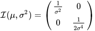
- La matriz de información de Fisher para una distribución normal con respecto a y es diagonal y toma la forma
- La distribución conjugada anterior de la media de una distribución normal es otra distribución normal. [35] Específicamente, si son iid y la distribución anterior es , entonces la distribución posterior para el estimador de será
- La familia de distribuciones normales no solo forma una familia exponencial (EF), sino que de hecho forma una familia exponencial natural (NEF) con función de varianza cuadrática ( NEF-QVF ). Muchas propiedades de las distribuciones normales se generalizan a propiedades de las distribuciones NEF-QVF, distribuciones NEF o distribuciones EF en general. Las distribuciones NEF-QVF comprenden 6 familias, incluidas las distribuciones Poisson, Gamma, binomial y binomial negativa, mientras que muchas de las familias comunes estudiadas en probabilidad y estadística son NEF o EF.
- En geometría de la información , la familia de distribuciones normales forma una variedad estadística con curvatura constante . La misma familia es plana con respecto a las conexiones (±1) y . [36]
- Si se distribuyen según , entonces . Nótese que no hay ningún supuesto de independencia. [37]








![{\textstyle E[\max _{i}X_{i}]\leq \sigma {\sqrt {2\ln n}}}](https://wikimedia.org/api/rest_v1/media/math/render/svg/0dfb87c9b047ccf23ace2139d97810dff1ed6670)
Distribuciones relacionadas
Teorema del límite central


El teorema del límite central establece que, en determinadas condiciones (bastante comunes), la suma de muchas variables aleatorias tendrá una distribución aproximadamente normal. Más específicamente, donde son variables aleatorias independientes e idénticamente distribuidas con la misma distribución arbitraria, media y varianza cero y su media está escalada por Entonces, a medida que aumenta, la distribución de probabilidad de tenderá a la distribución normal con media y varianza cero .


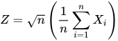
El teorema puede extenderse a variables que no son independientes y/o no están distribuidas idénticamente si se imponen ciertas restricciones al grado de dependencia y a los momentos de las distribuciones.

Muchas estadísticas de prueba , puntuaciones y estimadores que se encuentran en la práctica contienen sumas de ciertas variables aleatorias, e incluso más estimadores pueden representarse como sumas de variables aleatorias mediante el uso de funciones de influencia . El teorema del límite central implica que esos parámetros estadísticos tendrán distribuciones asintóticamente normales.
El teorema del límite central también implica que ciertas distribuciones pueden aproximarse mediante la distribución normal, por ejemplo:
- La distribución binomial es aproximadamente normal con media y varianza grandes y no demasiado cercanas a 0 o 1.
- La distribución de Poisson con parámetro es aproximadamente normal con media y varianza , para valores grandes de . [38]
- La distribución de chi-cuadrado es aproximadamente normal con media y varianza , para valores grandes .
- La distribución t de Student es aproximadamente normal con media 0 y varianza 1 cuando es grande.


La precisión de estas aproximaciones depende del propósito para el que se necesitan y de la tasa de convergencia a la distribución normal. Normalmente, estas aproximaciones son menos precisas en los extremos de la distribución.
El teorema de Berry-Esseen proporciona un límite superior general para el error de aproximación en el teorema del límite central y las expansiones de Edgeworth proporcionan mejoras en la aproximación .
Este teorema también se puede utilizar para justificar la modelización de la suma de muchas fuentes de ruido uniformes como ruido gaussiano . Véase AWGN .
Operaciones y funciones de variables normales


La densidad de probabilidad , la distribución acumulativa y la distribución acumulativa inversa de cualquier función de una o más variables normales independientes o correlacionadas se pueden calcular con el método numérico de trazado de rayos [39] (código Matlab). En las siguientes secciones, analizamos algunos casos especiales.
Operaciones sobre una sola variable normal
Si se distribuye normalmente con media y varianza , entonces
- , para cualquier número real y , también se distribuye normalmente, con media y varianza . Es decir, la familia de distribuciones normales está cerrada ante transformaciones lineales .
- La exponencial de se distribuye log-normalmente : .
- La sigmoide estándar de tiene una distribución logit-normal : .
- El valor absoluto de tiene una distribución normal plegada : . Si esto se conoce como distribución seminormal .
- El valor absoluto de los residuos normalizados, , tiene distribución chi con un grado de libertad: .
- El cuadrado de tiene una distribución chi-cuadrado no central con un grado de libertad: . Si , la distribución se denomina simplemente chi-cuadrado .
- La verosimilitud logarítmica de una variable normal es simplemente el logaritmo de su función de densidad de probabilidad : dado que se trata de un cuadrado escalado y desplazado de una variable normal estándar, se distribuye como una variable chi-cuadrado escalada y desplazada.
- La distribución de la variable restringida a un intervalo se denomina distribución normal truncada .
- tiene una distribución de Lévy con ubicación 0 y escala .






Operaciones sobre dos variables normales independientes
- Si y son dos variables aleatorias normales independientes , con medias , y varianzas , , entonces su suma también se distribuirá normalmente, [prueba] con media y varianza .
- En particular, si y son desviaciones normales independientes con media y varianza cero , entonces y también son independientes y se distribuyen normalmente, con media y varianza cero . Este es un caso especial de la identidad de polarización . [40]
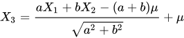
- Si , son dos desviaciones normales independientes con media y varianza , y , son números reales arbitrarios, entonces la variable también se distribuye normalmente con media y varianza . De ello se deduce que la distribución normal es estable (con exponente ).
- Si , son distribuciones normales, entonces su media geométrica normalizada es una distribución normal con y (ver aquí para una visualización).




Operaciones sobre dos variables normales estándar independientes
Si y son dos variables aleatorias normales estándar independientes con media 0 y varianza 1, entonces
- Su suma y diferencia se distribuyen normalmente con media cero y varianza dos: .
- Su producto sigue la distribución de producto [41] con función de densidad donde es la función de Bessel modificada de segundo tipo . Esta distribución es simétrica alrededor de cero, ilimitada en , y tiene la función característica .
- Su relación sigue la distribución estándar de Cauchy : .
- Su norma euclidiana tiene la distribución de Rayleigh .


Operaciones sobre múltiples variables normales independientes
- Cualquier combinación lineal de desviaciones normales independientes es una desviación normal.
- Si son variables aleatorias normales estándar independientes, entonces la suma de sus cuadrados tiene la distribución de chi-cuadrado con grados de libertad.
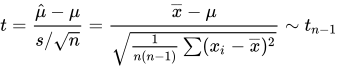
- Si son variables aleatorias independientes distribuidas normalmente con medias y varianzas , entonces su media muestral es independiente de la desviación estándar muestral , [42] lo que se puede demostrar utilizando el teorema de Basu o el teorema de Cochran . [43] La relación de estas dos cantidades tendrá la distribución t de Student con grados de libertad:
- Si , son variables aleatorias normales estándar independientes, entonces la relación de sus sumas de cuadrados normalizadas tendrá la distribución F con ( n , m ) grados de libertad: [44]



![{\displaystyle t={\frac {{\overline {X}}-\mu }{S/{\sqrt {n}}}}={\frac {{\frac {1}{n}}(X_{1}+\cdots +X_{n})-\mu }{\sqrt {{\frac {1}{n(n-1)}}\left[(X_{1}-{\overline {X}})^{2}+\cdots +(X_{n}-{\overline {X}})^{2}\right]}}}\sim t_{n-1}.}](https://wikimedia.org/api/rest_v1/media/math/render/svg/36ff0d3c79a0504e8f259ef99192b825357914d7)


Operaciones sobre múltiples variables normales correlacionadas
- Una forma cuadrática de un vector normal, es decir, una función cuadrática de múltiples variables normales independientes o correlacionadas, es una variable de chi-cuadrado generalizada .

Operaciones sobre la función de densidad
La distribución normal dividida se define de manera más directa en términos de unir secciones escaladas de las funciones de densidad de diferentes distribuciones normales y reescalar la densidad para integrarla en una sola. La distribución normal truncada resulta de reescalar una sección de una sola función de densidad.
Divisibilidad infinita y teorema de Cramér
Para cualquier entero positivo , cualquier distribución normal con media y varianza es la distribución de la suma de desviaciones normales independientes, cada una con media y varianza . Esta propiedad se llama divisibilidad infinita . [45]


Por el contrario, si y son variables aleatorias independientes y su suma tiene una distribución normal, entonces tanto como deben ser desviaciones normales. [46]
Este resultado se conoce como teorema de descomposición de Cramér y equivale a decir que la convolución de dos distribuciones es normal si y solo si ambas son normales. El teorema de Cramér implica que una combinación lineal de variables independientes no gaussianas nunca tendrá una distribución exactamente normal, aunque puede aproximarse a ella de forma arbitraria. [31]
El teorema de Kac-Bernstein
El teorema de Kac-Bernstein establece que si y son independientes y y también son independientes, entonces tanto X como Y deben tener necesariamente distribuciones normales. [47] [48]
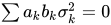
De manera más general, si son variables aleatorias independientes, entonces dos combinaciones lineales distintas y serán independientes si y solo si todas son normales y , donde denota la varianza de . [47]



Extensiones
El concepto de distribución normal, una de las distribuciones más importantes en la teoría de la probabilidad, se ha extendido mucho más allá del marco estándar del caso univariado (es decir, unidimensional) (caso 1). Todas estas extensiones también se denominan leyes normales o gaussianas , por lo que existe cierta ambigüedad en los nombres.
- La distribución normal multivariante describe la ley de Gauss en el espacio euclidiano de dimensión k . Un vector X ∈ R k tiene una distribución normal multivariante si cualquier combinación lineal de sus componentes Σkj =
1a j X j tiene una distribución normal (univariada). La varianza de X es unamatriz positiva definida simétrica k×k V . La distribución normal multivariada es un caso especial de las distribuciones elípticas . Como tal, sus lugares de isodensidad en el caso k = 2 son elipses y en el caso de k arbitrario son elipsoides . - Distribución gaussiana rectificada: una versión rectificada de la distribución normal con todos los elementos negativos restablecidos a 0.
- La distribución normal compleja se ocupa de los vectores normales complejos. Se dice que un vector complejo X ∈ C k es normal si sus componentes reales e imaginarios poseen conjuntamente una distribución normal multivariante de 2 k dimensiones. La estructura de varianza-covarianza de X se describe mediante dos matrices: la matriz de varianza Γ y la matriz de relación C .
- La distribución normal matricial describe el caso de matrices distribuidas normalmente.
- Los procesos gaussianos son procesos estocásticos distribuidos normalmente . Estos pueden verse como elementos de algún espacio de Hilbert de dimensión infinita H y, por lo tanto, son los análogos de los vectores normales multivariados para el caso k = ∞ . Se dice que un elemento aleatorio h ∈ H es normal si para cualquier constante a ∈ H el producto escalar ( a , h ) tiene una distribución normal (univariada). La estructura de varianza de dicho elemento aleatorio gaussiano puede describirse en términos del operador de covarianza lineal K: H → H . Varios procesos gaussianos se hicieron lo suficientemente populares como para tener sus propios nombres:
- movimiento browniano
- Puente browniano
- Proceso de Ornstein-Uhlenbeck .
- La distribución q gaussiana es una construcción matemática abstracta que representa un análogo q de la distribución normal.
- La distribución q-gaussiana es análoga a la distribución gaussiana, en el sentido de que maximiza la entropía de Tsallis y es un tipo de distribución de Tsallis . Esta distribución es diferente de la distribución q gaussiana anterior.
- La distribución κ -Gaussiana de Kaniadakis es una generalización de la distribución Gaussiana que surge de las estadísticas de Kaniadakis , siendo una de las distribuciones de Kaniadakis .
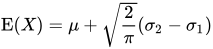
Una variable aleatoria X tiene una distribución normal de dos piezas si tiene una distribución


donde μ es la media y σ 1 2 y σ 2 2 son las varianzas de la distribución a la izquierda y a la derecha de la media respectivamente.
Se han determinado la media, la varianza y el tercer momento central de esta distribución [49]

![{\displaystyle \operatorname {T} (X)={\sqrt {\frac {2}{\pi }}}(\sigma _{2}-\sigma _{1})\left[\left({\frac {4}{\pi }}-1\right)(\sigma _{2}-\sigma _{1})^{2}+\sigma _{1}\sigma _{2}\right]}](https://wikimedia.org/api/rest_v1/media/math/render/svg/9959f2c5186e2ed76884054edaf837a602ac6fac)
donde E( X ), V( X ) y T( X ) son la media, la varianza y el tercer momento central respectivamente.
Uno de los principales usos prácticos de la ley de Gauss es modelar las distribuciones empíricas de muchas variables aleatorias diferentes que se encuentran en la práctica. En tal caso, una posible extensión sería una familia más rica de distribuciones, que tuviera más de dos parámetros y, por lo tanto, pudiera ajustarse a la distribución empírica con mayor precisión. Los ejemplos de tales extensiones son:
- Distribución de Pearson : una familia de distribuciones de probabilidad de cuatro parámetros que extienden la ley normal para incluir diferentes valores de asimetría y curtosis.
- La distribución normal generalizada , también conocida como distribución de potencia exponencial, permite colas de distribución con comportamientos asintóticos más gruesos o más delgados.
Inferencia estadística
Estimación de parámetros
A menudo sucede que no conocemos los parámetros de la distribución normal, pero queremos estimarlos . Es decir, si tenemos una muestra de una población normal, nos gustaría conocer los valores aproximados de los parámetros y . El enfoque estándar para este problema es el método de máxima verosimilitud , que requiere maximizar la función de log-verosimilitud : Tomando derivadas con respecto a y y resolviendo el sistema resultante de condiciones de primer orden se obtienen las estimaciones de máxima verosimilitud :



Entonces es como sigue:

![{\displaystyle \ln {\mathcal {L}}({\hat {\mu }},{\hat {\sigma }}^{2})=(-n/2)[\ln(2\pi {\hat {\sigma }}^{2})+1]}](https://wikimedia.org/api/rest_v1/media/math/render/svg/561353e6bc80d226fddd9510be61d21bc67b3aee)
Media de la muestra
El estimador se denomina media muestral , ya que es la media aritmética de todas las observaciones. La estadística es completa y suficiente para , y por lo tanto, por el teorema de Lehmann-Scheffé , es el estimador insesgado de varianza mínima uniforme (UMVU). [50] En muestras finitas se distribuye normalmente: La varianza de este estimador es igual al elemento μμ de la matriz de información de Fisher inversa . Esto implica que el estimador es eficiente en muestras finitas . De importancia práctica es el hecho de que el error estándar de es proporcional a , es decir, si uno desea disminuir el error estándar en un factor de 10, uno debe aumentar el número de puntos en la muestra en un factor de 100. Este hecho se usa ampliamente para determinar los tamaños de muestra para encuestas de opinión y el número de ensayos en simulaciones de Monte Carlo .





Desde el punto de vista de la teoría asintótica , es consistente , es decir, converge en probabilidad a cuando . El estimador también es asintóticamente normal , lo que es un corolario simple del hecho de que es normal en muestras finitas:


Varianza de la muestra
El estimador se denomina varianza muestral , ya que es la varianza de la muestra ( ). En la práctica, a menudo se utiliza otro estimador en lugar del . Este otro estimador se denota , y también se denomina varianza muestral , lo que representa una cierta ambigüedad en la terminología; su raíz cuadrada se denomina desviación estándar muestral . El estimador se diferencia de por tener ( n − 1) en lugar de n en el denominador (la llamada corrección de Bessel ): La diferencia entre y se vuelve insignificantemente pequeña para n grandes . Sin embargo, en muestras finitas, la motivación detrás del uso de es que es un estimador insesgado del parámetro subyacente , mientras que está sesgado. Además, por el teorema de Lehmann-Scheffé, el estimador es uniformemente de varianza mínima insesgado ( UMVU ), [50] lo que lo convierte en el "mejor" estimador entre todos los insesgados. Sin embargo, se puede demostrar que el estimador sesgado es mejor que el en términos del criterio del error cuadrático medio (MSE). En muestras finitas, tanto y tienen una distribución chi-cuadrado escalada con ( n − 1) grados de libertad: La primera de estas expresiones muestra que la varianza de es igual a , que es ligeramente mayor que el elemento σσ de la matriz de información de Fisher inversa . Por lo tanto, no es un estimador eficiente para , y además, dado que es UMVU, podemos concluir que el estimador eficiente de muestra finita para no existe.





Aplicando la teoría asintótica, ambos estimadores y son consistentes, es decir, convergen en probabilidad a cuando el tamaño de la muestra es . Los dos estimadores también son asintóticamente normales: En particular, ambos estimadores son asintóticamente eficientes para .

Intervalos de confianza
Por el teorema de Cochran , para distribuciones normales la media muestral y la varianza muestral s 2 son independientes , lo que significa que no puede haber ganancia en considerar su distribución conjunta . También hay un teorema inverso: si en una muestra la media muestral y la varianza muestral son independientes, entonces la muestra debe provenir de la distribución normal. La independencia entre y s se puede emplear para construir el llamado estadístico t :
Esta cantidad t tiene la distribución t de Student con ( n − 1) grados de libertad, y es un estadístico auxiliar (independiente del valor de los parámetros). Invertir la distribución de este estadístico t nos permitirá construir el intervalo de confianza para μ ; [51] de manera similar, invertir la distribución χ 2 del estadístico s 2 nos dará el intervalo de confianza para σ 2 : [52]
donde t k,p y χ
2
k,p son los cuantiles p de las distribuciones t y χ 2 , respectivamente. Estos intervalos de confianza tienen un nivel de confianza de 1 − α , lo que significa que los valores verdaderos μ y σ 2 quedan fuera de estos intervalos con una probabilidad (o nivel de significancia ) α . En la práctica, la gente suele tomar α = 5% , lo que da como resultado intervalos de confianza del 95%. El intervalo de confianza para σ se puede encontrar tomando la raíz cuadrada de los límites del intervalo para σ 2 .
![{\displaystyle \mu \in \left[{\hat {\mu }}-{\frac {t_{n-1,1-\alpha /2}}{\sqrt {n}}}s,\,{\hat {\mu }}+{\frac {t_{n-1,1-\alpha /2}}{\sqrt {n}}}s\right],}](https://wikimedia.org/api/rest_v1/media/math/render/svg/1e0b267730af48c4a13b2947e1ee41bd828f92eb)
![{\displaystyle \sigma ^{2}\in \left[{\frac {n-1}{\chi _{n-1,1-\alpha /2}^{2}}}s^{2},\,{\frac {n-1}{\chi _{n-1,\alpha /2}^{2}}}s^{2}\right],}](https://wikimedia.org/api/rest_v1/media/math/render/svg/4a8fc65b99199a5894b71f3089dc1643322dd875)
Se pueden derivar fórmulas aproximadas a partir de las distribuciones asintóticas de y s 2 : Las fórmulas aproximadas se vuelven válidas para valores grandes de n , y son más convenientes para el cálculo manual ya que los cuantiles normales estándar z α /2 no dependen de n . En particular, el valor más popular de α = 5% , da como resultado | z 0,025 | = 1,96 .
![{\displaystyle \mu \in \left[{\hat {\mu }}-{\frac {|z_{\alpha /2}|}{\sqrt {n}}}s,\,{\hat {\mu }}+{\frac {|z_{\alpha /2}|}{\sqrt {n}}}s\right],}](https://wikimedia.org/api/rest_v1/media/math/render/svg/8aeaa29c4240ae0df25b32b05941ea7548e9e4dd)
![{\displaystyle \sigma ^{2}\in \left[s^{2}-{\sqrt {2}}{\frac {|z_{\alpha /2}|}{\sqrt {n}}}s^{2},\,s^{2}+{\sqrt {2}}{\frac {|z_{\alpha /2}|}{\sqrt {n}}}s^{2}\right],}](https://wikimedia.org/api/rest_v1/media/math/render/svg/a019ba33d7f994b3e3bf95f65a69db767894a3cb)
Pruebas de normalidad
Las pruebas de normalidad evalúan la probabilidad de que el conjunto de datos dado { x 1 , ..., x n } provenga de una distribución normal. Normalmente, la hipótesis nula H 0 es que las observaciones se distribuyen normalmente con una media μ y una varianza σ 2 no especificadas , frente a la alternativa H a de que la distribución es arbitraria. Se han ideado muchas pruebas (más de 40) para este problema. Las más destacadas se describen a continuación:
Los gráficos de diagnóstico son más atractivos intuitivamente, pero subjetivos al mismo tiempo, ya que se basan en el juicio humano informal para aceptar o rechazar la hipótesis nula.
- El gráfico Q–Q , también conocido como gráfico de probabilidad normal o gráfico de Rankit , es un gráfico de los valores ordenados del conjunto de datos contra los valores esperados de los cuantiles correspondientes de la distribución normal estándar. Es decir, es un gráfico de puntos de la forma (Φ −1 ( p k ), x ( k ) ), donde los puntos de trazado p k son iguales a p k = ( k − α )/( n + 1 − 2 α ) y α es una constante de ajuste, que puede ser cualquier valor entre 0 y 1. Si la hipótesis nula es verdadera, los puntos trazados deben estar aproximadamente en una línea recta.
- Diagrama P–P : similar al diagrama Q–Q, pero usado con mucha menos frecuencia. Este método consiste en representar gráficamente los puntos (Φ( z ( k ) ), p k ), donde . Para datos distribuidos normalmente, este diagrama debe estar en una línea de 45° entre (0, 0) y (1, 1).

Pruebas de bondad de ajuste :
Pruebas basadas en momentos :
- Prueba del K-cuadrado de D'Agostino
- Prueba de Jarque-Bera
- Prueba de Shapiro-Wilk : se basa en el hecho de que la línea en el gráfico Q-Q tiene una pendiente de σ . La prueba compara la estimación de mínimos cuadrados de esa pendiente con el valor de la varianza de la muestra y rechaza la hipótesis nula si estas dos cantidades difieren significativamente.
Pruebas basadas en la función de distribución empírica :
- Prueba de Anderson-Darling
- Prueba de Lilliefors (una adaptación de la prueba de Kolmogorov-Smirnov )
Análisis bayesiano de la distribución normal
El análisis bayesiano de datos distribuidos normalmente se complica por las muchas posibilidades diferentes que pueden considerarse:
- Tanto la media como la varianza, o ninguna de ellas, pueden considerarse una cantidad fija.
- Cuando se desconoce la varianza, el análisis puede realizarse directamente en términos de la varianza o en términos de la precisión , el recíproco de la varianza. La razón para expresar las fórmulas en términos de precisión es que se simplifica el análisis de la mayoría de los casos.
- Es necesario considerar tanto los casos univariados como los multivariados .
- Se pueden colocar distribuciones previas conjugadas o impropias en las variables desconocidas.
- En la regresión lineal bayesiana se da un conjunto adicional de casos , en los que en el modelo básico se supone que los datos se distribuyen normalmente y se aplican valores a priori normales a los coeficientes de regresión . El análisis resultante es similar a los casos básicos de datos independientes distribuidos de forma idéntica .
Las fórmulas para los casos de regresión no lineal se resumen en el artículo anterior conjugado .
Suma de dos cuadráticas
Forma escalar
La siguiente fórmula auxiliar es útil para simplificar las ecuaciones de actualización posterior , que de otro modo se vuelven bastante tediosas.

Esta ecuación reescribe la suma de dos ecuaciones cuadráticas en x expandiendo los cuadrados, agrupando los términos en x y completando el cuadrado . Tenga en cuenta lo siguiente sobre los factores constantes complejos asociados a algunos de los términos:
- El factor tiene la forma de un promedio ponderado de y y z .
- Esto demuestra que este factor puede considerarse como el resultado de una situación en la que los recíprocos de las cantidades a y b se suman directamente, por lo que para combinar a y b , es necesario recíprocar, sumar y recíprocar el resultado nuevamente para volver a las unidades originales. Este es exactamente el tipo de operación que realiza la media armónica , por lo que no es sorprendente que sea la mitad de la media armónica de a y b .


Forma vectorial
Se puede escribir una fórmula similar para la suma de dos cuadráticas vectoriales: Si x , y , z son vectores de longitud k , y A y B son matrices simétricas e invertibles de tamaño , entonces


dónde

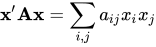
La forma x ′ A x se llama forma cuadrática y es un escalar : En otras palabras, suma todas las combinaciones posibles de productos de pares de elementos de x , con un coeficiente separado para cada uno. Además, como , solo importa la suma para cualquier elemento fuera de la diagonal de A , y no hay pérdida de generalidad al suponer que A es simétrico . Además, si A es simétrico, entonces la forma


Suma de las diferencias con respecto a la media
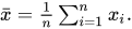
Otra fórmula útil es la siguiente: donde

Con varianza conocida
Para un conjunto de puntos de datos iid distribuidos normalmente X de tamaño n , donde cada punto individual x sigue con una varianza conocida σ 2 , la distribución previa conjugada también se distribuye normalmente.

Esto se puede demostrar más fácilmente reescribiendo la varianza como la precisión , es decir, utilizando τ = 1/σ 2 . Entonces, si y procedemos de la siguiente manera.


En primer lugar, la función de probabilidad es (usando la fórmula anterior para la suma de las diferencias con respecto a la media):
![{\displaystyle {\begin{aligned}p(\mathbf {X} \mid \mu ,\tau )&=\prod _{i=1}^{n}{\sqrt {\frac {\tau }{2\pi }}}\exp \left(-{\frac {1}{2}}\tau (x_{i}-\mu )^{2}\right)\\&=\left({\frac {\tau }{2\pi }}\right)^{n/2}\exp \left(-{\frac {1}{2}}\tau \sum _{i=1}^{n}(x_{i}-\mu )^{2}\right)\\&=\left({\frac {\tau }{2\pi }}\right)^{n/2}\exp \left[-{\frac {1}{2}}\tau \left(\sum _{i=1}^{n}(x_{i}-{\bar {x}})^{2}+n({\bar {x}}-\mu )^{2}\right)\right].\end{alineado}}}](https://wikimedia.org/api/rest_v1/media/math/render/svg/c2bcd1c34520a24e29b758a0f7427e79e9d8a414)
Luego procedemos de la siguiente manera:
![{\displaystyle {\begin{aligned}p(\mu \mid \mathbf {X} )&\propto p(\mathbf {X} \mid \mu )p(\mu )\\&=\left({\frac {\tau }{2\pi }}\right)^{n/2}\exp \left[-{\frac {1}{2}}\tau \left(\sum _{i=1}^{n}(x_{i}-{\bar {x}})^{2}+n({\bar {x}}-\mu )^{2}\right)\right]{\sqrt {\frac {\tau _{0}}{2\pi }}}\exp \left(-{\frac {1}{2}}\tau _{0}(\mu -\mu _{0})^{2}\right)\\&\propto \exp \left(-{\frac {1}{2}}(\tau \left(\sum _{i=1}^{n}(x_{i}-{\bar {x}})^{2}+n({\bar {x}}-\mu )^{2}\right)+\tau _{0}(\mu -\mu _{0})^{2}\right)\right)\\&\propto \exp \left(-{\frac {1}{2}}(n\tau ({\bar {x}}-\mu )^{2}+\tau _{0}(\mu -\mu _{0})^{2}\right)\right)\\&=\exp \left(-{\frac {1}{2}}(n\tau +\tau _{0})\left(\mu -{\dfrac {n\tau {\bar {x}}+\tau _{0}\mu _{0}}{n\tau +\tau _{0}}}\right)^{2}+{\frac {n\tau \tau _{0}}{n\tau +\tau _{0}}}({\bar {x}}-\mu _{0})^{2}\right)\\&\propto \exp \left(-{\frac {1}{2}}(n\tau +\tau _{0})\left(\mu -{\dfrac {n\tau {\bar {x}}+\tau _{0}\mu _{0}}{n\tau +\tau _{0}}}\right)^{2}\right)\end{aligned}}}](https://wikimedia.org/api/rest_v1/media/math/render/svg/96e309ead00fbc8603eced5342aa5df534522d6a)
En la derivación anterior, utilizamos la fórmula anterior para la suma de dos cuadráticas y eliminamos todos los factores constantes que no involucran μ . El resultado es el núcleo de una distribución normal, con media y precisión , es decir



Esto se puede escribir como un conjunto de ecuaciones de actualización bayesianas para los parámetros posteriores en términos de los parámetros anteriores:
![{\displaystyle {\begin{aligned}\tau _{0}'&=\tau _{0}+n\tau \\[5pt]\mu _{0}'&={\frac {n\tau {\bar {x}}+\tau _{0}\mu _{0}}{n\tau +\tau _{0}}}\\[5pt]{\bar {x}}&={\frac {1}{n}}\sum _{i=1}^{n}x_{i}\end{aligned}}}](https://wikimedia.org/api/rest_v1/media/math/render/svg/a6cfbdf504b1a9ce4cbe79561b4ae983fdf7271d)
Es decir, combinar n puntos de datos con precisión total de nτ (o equivalentemente, varianza total de n / σ 2 ) y media de valores , derivar una nueva precisión total simplemente sumando la precisión total de los datos a la precisión total previa, y formar una nueva media a través de un promedio ponderado por precisión , es decir, un promedio ponderado de la media de los datos y la media previa, cada una ponderada por la precisión total asociada. Esto tiene sentido lógico si se piensa que la precisión indica la certeza de las observaciones: en la distribución de la media posterior, cada uno de los componentes de entrada está ponderado por su certeza, y la certeza de esta distribución es la suma de las certezas individuales. (Para la intuición de esto, compare la expresión "el todo es (o no es) mayor que la suma de sus partes". Además, considere que el conocimiento de la posterior proviene de una combinación del conocimiento de la anterior y la probabilidad, por lo que tiene sentido que estemos más seguros de él que de cualquiera de sus componentes).

La fórmula anterior revela por qué es más conveniente realizar un análisis bayesiano de valores anteriores conjugados para la distribución normal en términos de precisión. La precisión posterior es simplemente la suma de las precisiones anterior y de probabilidad, y la media posterior se calcula a través de un promedio ponderado por precisión, como se describió anteriormente. Las mismas fórmulas se pueden escribir en términos de varianza al reciprocar todas las precisiones, lo que produce las fórmulas más feas.
![{\displaystyle {\begin{aligned}{\sigma _{0}^{2}}'&={\frac {1}{{\frac {n}{\sigma ^{2}}}+{\frac {1}{\sigma _{0}^{2}}}}\\[5pt]\mu _{0}'&={\frac {{\frac {n{\bar {x}}}{\sigma ^{2}}}+{\frac {\mu _{0}}{\sigma _{0}^{2}}}}{{\frac {n}{\sigma ^{2}}}+{\frac {1}{\sigma _{0}^{2}}}}}\\[5pt]{\bar {x}}&={\frac {1}{n}}\sum _{i=1}^{n}x_{i}\end{aligned}}}](https://wikimedia.org/api/rest_v1/media/math/render/svg/ea454c8840683777ce8192d9ae63068c63962858)
Con media conocida
Para un conjunto de puntos de datos distribuidos normalmente iid X de tamaño n donde cada punto individual x sigue con media conocida μ, la distribución previa conjugada de la varianza tiene una distribución gamma inversa o una distribución chi-cuadrado inversa escalada . Las dos son equivalentes excepto por tener diferentes parametrizaciones . Aunque la gamma inversa se usa más comúnmente, usamos la chi-cuadrado inversa escalada por conveniencia. La distribución previa para σ 2 es la siguiente:
![{\displaystyle p(\sigma ^{2}\mid \nu _{0},\sigma _{0}^{2})={\frac {(\sigma _{0}^{2}{\frac {\nu _{0}}{2}})^{\nu _{0}/2}}{\Gamma \left({\frac {\nu _{0}}{2}}\right)}}~{\frac {\exp \left[{\frac {-\nu _{0}\sigma _{0}^{2}}{2\sigma ^{2}}}\right]}{(\sigma ^{2})^{1+{\frac {\nu _{0}}{2}}}}\propto {\frac {\exp \left[{\frac {-\nu _{0}\sigma _{0}^{2}}{2\sigma ^{2}}}\right]}{(\sigma ^{2})^{1+{\frac {\nu _{0}}{2}}}}}}](https://wikimedia.org/api/rest_v1/media/math/render/svg/ef2528fe4774a93087d4adae570ef9ab84707f52)
La función de probabilidad de arriba, escrita en términos de la varianza, es:
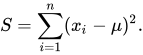
![{\displaystyle {\begin{aligned}p(\mathbf {X} \mid \mu ,\sigma ^{2})&=\left({\frac {1}{2\pi \sigma ^{2}}}\right)^{n/2}\exp \left[-{\frac {1}{2\sigma ^{2}}}\sum _{i=1}^{n}(x_{i}-\mu )^{2}\right]\\&=\left({\frac {1}{2\pi \sigma ^{2}}}\right)^{n/2}\exp \left[-{\frac {S}{2\sigma ^{2}}}\right]\end{aligned}}}](https://wikimedia.org/api/rest_v1/media/math/render/svg/cc06aa31588bba03e4748f8f345f0638a75dc156)
dónde
Entonces:
![{\displaystyle {\begin{aligned}p(\sigma ^{2}\mid \mathbf {X} )&\propto p(\mathbf {X} \mid \sigma ^{2})p(\sigma ^{2})\\&=\left({\frac {1}{2\pi \sigma ^{2}}}\right)^{n/2}\exp \left[-{\frac {S}{2\sigma ^{2}}}\right]{\frac {(\sigma _{0}^{2}{\frac {\nu _{0}}{2}})^{\frac {\nu _{0}}{2}}}{\Gamma \left({\frac {\nu _{0}}{2}}\right)}}~{\frac {\exp \left[{\frac {-\nu _{0}\sigma _{0}^{2}}{2\sigma ^{2}}}\derecha]}{(\sigma ^{2})^{1+{\frac {\nu _{0}}{2}}}}}\\&\propto \izquierda({\frac {1}{\sigma ^{2}}}\derecha)^{n/2}{\frac {1}{(\sigma ^{2})^{1+{\frac {\nu _{0}}{2}}}}}\exp \izquierda[-{\frac {S}{2\sigma ^{2}}}+{\frac {-\nu _{0}\sigma _{0}^{2}}{2\sigma ^{2}}}\derecha]\\&={\frac {1}{(\sigma ^{2})^{1+{\frac {\nu _{0}+n}{2}}}}}\exp \izquierda[-{\frac {\nu _{0}\sigma _{0}^{2}+S}{2\sigma ^{2}}}\derecha]\end{alineado}}}](https://wikimedia.org/api/rest_v1/media/math/render/svg/381c1b93f6dc76e2cdca9f3f1f77132dd51dc55f)
Lo anterior también es una distribución chi-cuadrado inversa escalada donde
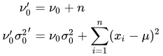
o equivalentemente
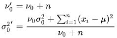
Reparametrizando en términos de una distribución gamma inversa , el resultado es:
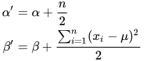
Con media desconocida y varianza desconocida
Para un conjunto de puntos de datos distribuidos normalmente iid X de tamaño n donde cada punto individual x sigue con media desconocida μ y varianza desconocida σ 2 , se coloca una distribución previa conjugada combinada (multivariada) sobre la media y la varianza, que consiste en una distribución gamma inversa normal . Lógicamente, esto se origina de la siguiente manera:
- A partir del análisis del caso con media desconocida pero varianza conocida, vemos que las ecuaciones de actualización involucran estadísticas suficientes calculadas a partir de los datos que consisten en la media de los puntos de datos y la varianza total de los puntos de datos, calculada a su vez a partir de la varianza conocida dividida por el número de puntos de datos.
- A partir del análisis del caso con varianza desconocida pero media conocida, vemos que las ecuaciones de actualización involucran estadísticas suficientes sobre los datos que consisten en el número de puntos de datos y la suma de las desviaciones al cuadrado .
- Tenga en cuenta que los valores de actualización posteriores sirven como distribución a priori cuando se manejan más datos. Por lo tanto, lógicamente deberíamos pensar en nuestros valores a priori en términos de las estadísticas suficientes que acabamos de describir, teniendo en cuenta la misma semántica tanto como sea posible.
- Para manejar el caso en el que tanto la media como la varianza son desconocidas, podríamos colocar valores a priori independientes sobre la media y la varianza, con estimaciones fijas de la media promedio, la varianza total, el número de puntos de datos utilizados para calcular el valor a priori de la varianza y la suma de las desviaciones al cuadrado. Sin embargo, tenga en cuenta que, en realidad, la varianza total de la media depende de la varianza desconocida, y la suma de las desviaciones al cuadrado que entran en el valor a priori de la varianza (parece) depende de la media desconocida. En la práctica, esta última dependencia es relativamente poco importante: al cambiar la media real, se cambian los puntos generados en una cantidad igual y, en promedio, las desviaciones al cuadrado permanecerán iguales. Sin embargo, este no es el caso con la varianza total de la media: a medida que aumenta la varianza desconocida, la varianza total de la media aumentará proporcionalmente y nos gustaría capturar esta dependencia.
- This suggests that we create a conditional prior of the mean on the unknown variance, with a hyperparameter specifying the mean of the pseudo-observations associated with the prior, and another parameter specifying the number of pseudo-observations. This number serves as a scaling parameter on the variance, making it possible to control the overall variance of the mean relative to the actual variance parameter. The prior for the variance also has two hyperparameters, one specifying the sum of squared deviations of the pseudo-observations associated with the prior, and another specifying once again the number of pseudo-observations. Each of the priors has a hyperparameter specifying the number of pseudo-observations, and in each case this controls the relative variance of that prior. These are given as two separate hyperparameters so that the variance (aka the confidence) of the two priors can be controlled separately.
- This leads immediately to the normal-inverse-gamma distribution, which is the product of the two distributions just defined, with conjugate priors used (an inverse gamma distribution over the variance, and a normal distribution over the mean, conditional on the variance) and with the same four parameters just defined.
The priors are normally defined as follows:

The update equations can be derived, and look as follows:
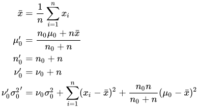
The respective numbers of pseudo-observations add the number of actual observations to them. The new mean hyperparameter is once again a weighted average, this time weighted by the relative numbers of observations. Finally, the update for is similar to the case with known mean, but in this case the sum of squared deviations is taken with respect to the observed data mean rather than the true mean, and as a result a new interaction term needs to be added to take care of the additional error source stemming from the deviation between prior and data mean.

The prior distributions are
![{\displaystyle {\begin{aligned}p(\mu \mid \sigma ^{2};\mu _{0},n_{0})&\sim {\mathcal {N}}(\mu _{0},\sigma ^{2}/n_{0})={\frac {1}{\sqrt {2\pi {\frac {\sigma ^{2}}{n_{0}}}}}}\exp \left(-{\frac {n_{0}}{2\sigma ^{2}}}(\mu -\mu _{0})^{2}\right)\\&\propto (\sigma ^{2})^{-1/2}\exp \left(-{\frac {n_{0}}{2\sigma ^{2}}}(\mu -\mu _{0})^{2}\right)\\p(\sigma ^{2};\nu _{0},\sigma _{0}^{2})&\sim I\chi ^{2}(\nu _{0},\sigma _{0}^{2})=IG(\nu _{0}/2,\nu _{0}\sigma _{0}^{2}/2)\\&={\frac {(\sigma _{0}^{2}\nu _{0}/2)^{\nu _{0}/2}}{\Gamma (\nu _{0}/2)}}~{\frac {\exp \left[{\frac {-\nu _{0}\sigma _{0}^{2}}{2\sigma ^{2}}}\right]}{(\sigma ^{2})^{1+\nu _{0}/2}}}\\&\propto {(\sigma ^{2})^{-(1+\nu _{0}/2)}}\exp \left[{\frac {-\nu _{0}\sigma _{0}^{2}}{2\sigma ^{2}}}\right].\end{aligned}}}](https://wikimedia.org/api/rest_v1/media/math/render/svg/cf7afb8e3b63fb1526171840344b32458e55cf8b)
Therefore, the joint prior is
![{\displaystyle {\begin{aligned}p(\mu ,\sigma ^{2};\mu _{0},n_{0},\nu _{0},\sigma _{0}^{2})&=p(\mu \mid \sigma ^{2};\mu _{0},n_{0})\,p(\sigma ^{2};\nu _{0},\sigma _{0}^{2})\\&\propto (\sigma ^{2})^{-(\nu _{0}+3)/2}\exp \left[-{\frac {1}{2\sigma ^{2}}}\left(\nu _{0}\sigma _{0}^{2}+n_{0}(\mu -\mu _{0})^{2}\right)\right].\end{aligned}}}](https://wikimedia.org/api/rest_v1/media/math/render/svg/b6f808161077baef3854dbfd90b870698d721090)
The likelihood function from the section above with known variance is:
![{\displaystyle {\begin{aligned}p(\mathbf {X} \mid \mu ,\sigma ^{2})&=\left({\frac {1}{2\pi \sigma ^{2}}}\right)^{n/2}\exp \left[-{\frac {1}{2\sigma ^{2}}}\left(\sum _{i=1}^{n}(x_{i}-\mu )^{2}\right)\right]\end{aligned}}}](https://wikimedia.org/api/rest_v1/media/math/render/svg/f3d77342aadcb34c5d84418cecaefdb52842b6b7)
Writing it in terms of variance rather than precision, we get: where
![{\displaystyle {\begin{aligned}p(\mathbf {X} \mid \mu ,\sigma ^{2})&=\left({\frac {1}{2\pi \sigma ^{2}}}\right)^{n/2}\exp \left[-{\frac {1}{2\sigma ^{2}}}\left(\sum _{i=1}^{n}(x_{i}-{\bar {x}})^{2}+n({\bar {x}}-\mu )^{2}\right)\right]\\&\propto {\sigma ^{2}}^{-n/2}\exp \left[-{\frac {1}{2\sigma ^{2}}}\left(S+n({\bar {x}}-\mu )^{2}\right)\right]\end{aligned}}}](https://wikimedia.org/api/rest_v1/media/math/render/svg/29b915f070b522a1e9f419be05624c86c854ca14)

Therefore, the posterior is (dropping the hyperparameters as conditioning factors):
![{\displaystyle {\begin{aligned}p(\mu ,\sigma ^{2}\mid \mathbf {X} )&\propto p(\mu ,\sigma ^{2})\,p(\mathbf {X} \mid \mu ,\sigma ^{2})\\&\propto (\sigma ^{2})^{-(\nu _{0}+3)/2}\exp \left[-{\frac {1}{2\sigma ^{2}}}\left(\nu _{0}\sigma _{0}^{2}+n_{0}(\mu -\mu _{0})^{2}\right)\right]{\sigma ^{2}}^{-n/2}\exp \left[-{\frac {1}{2\sigma ^{2}}}\left(S+n({\bar {x}}-\mu )^{2}\right)\right]\\&=(\sigma ^{2})^{-(\nu _{0}+n+3)/2}\exp \left[-{\frac {1}{2\sigma ^{2}}}\left(\nu _{0}\sigma _{0}^{2}+S+n_{0}(\mu -\mu _{0})^{2}+n({\bar {x}}-\mu )^{2}\right)\right]\\&=(\sigma ^{2})^{-(\nu _{0}+n+3)/2}\exp \left[-{\frac {1}{2\sigma ^{2}}}\left(\nu _{0}\sigma _{0}^{2}+S+{\frac {n_{0}n}{n_{0}+n}}(\mu _{0}-{\bar {x}})^{2}+(n_{0}+n)\left(\mu -{\frac {n_{0}\mu _{0}+n{\bar {x}}}{n_{0}+n}}\right)^{2}\right)\right]\\&\propto (\sigma ^{2})^{-1/2}\exp \left[-{\frac {n_{0}+n}{2\sigma ^{2}}}\left(\mu -{\frac {n_{0}\mu _{0}+n{\bar {x}}}{n_{0}+n}}\right)^{2}\right]\\&\quad \times (\sigma ^{2})^{-(\nu _{0}/2+n/2+1)}\exp \left[-{\frac {1}{2\sigma ^{2}}}\left(\nu _{0}\sigma _{0}^{2}+S+{\frac {n_{0}n}{n_{0}+n}}(\mu _{0}-{\bar {x}})^{2}\right)\right]\\&={\mathcal {N}}_{\mu \mid \sigma ^{2}}\left({\frac {n_{0}\mu _{0}+n{\bar {x}}}{n_{0}+n}},{\frac {\sigma ^{2}}{n_{0}+n}}\right)\cdot {\rm {IG}}_{\sigma ^{2}}\left({\frac {1}{2}}(\nu _{0}+n),{\frac {1}{2}}\left(\nu _{0}\sigma _{0}^{2}+S+{\frac {n_{0}n}{n_{0}+n}}(\mu _{0}-{\bar {x}})^{2}\right)\right).\end{aligned}}}](https://wikimedia.org/api/rest_v1/media/math/render/svg/cad9489034d77d53c12c7ee6044f712cfdb77831)
In other words, the posterior distribution has the form of a product of a normal distribution over times an inverse gamma distribution over , with parameters that are the same as the update equations above.


Occurrence and applications
The occurrence of normal distribution in practical problems can be loosely classified into four categories:
- Exactly normal distributions;
- Approximately normal laws, for example when such approximation is justified by the central limit theorem; and
- Distributions modeled as normal – the normal distribution being the distribution with maximum entropy for a given mean and variance.
- Regression problems – the normal distribution being found after systematic effects have been modeled sufficiently well.
Exact normality

Certain quantities in physics are distributed normally, as was first demonstrated by James Clerk Maxwell. Examples of such quantities are:
- Probability density function of a ground state in a quantum harmonic oscillator.
- The position of a particle that experiences diffusion. If initially the particle is located at a specific point (that is its probability distribution is the Dirac delta function), then after time t its location is described by a normal distribution with variance t, which satisfies the diffusion equation . If the initial location is given by a certain density function , then the density at time t is the convolution of g and the normal probability density function.


Approximate normality
Approximately normal distributions occur in many situations, as explained by the central limit theorem. When the outcome is produced by many small effects acting additively and independently, its distribution will be close to normal. The normal approximation will not be valid if the effects act multiplicatively (instead of additively), or if there is a single external influence that has a considerably larger magnitude than the rest of the effects.
- In counting problems, where the central limit theorem includes a discrete-to-continuum approximation and where infinitely divisible and decomposable distributions are involved, such as
- Binomial random variables, associated with binary response variables;
- Poisson random variables, associated with rare events;
- Thermal radiation has a Bose–Einstein distribution on very short time scales, and a normal distribution on longer timescales due to the central limit theorem.
Assumed normality
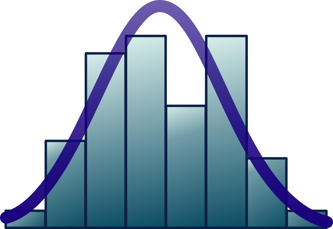
I can only recognize the occurrence of the normal curve – the Laplacian curve of errors – as a very abnormal phenomenon. It is roughly approximated to in certain distributions; for this reason, and on account for its beautiful simplicity, we may, perhaps, use it as a first approximation, particularly in theoretical investigations.
— Pearson (1901)
There are statistical methods to empirically test that assumption; see the above Normality tests section.
- In biology, the logarithm of various variables tend to have a normal distribution, that is, they tend to have a log-normal distribution (after separation on male/female subpopulations), with examples including:
- Measures of size of living tissue (length, height, skin area, weight);[53]
- The length of inert appendages (hair, claws, nails, teeth) of biological specimens, in the direction of growth; presumably the thickness of tree bark also falls under this category;
- Certain physiological measurements, such as blood pressure of adult humans.
- In finance, in particular the Black–Scholes model, changes in the logarithm of exchange rates, price indices, and stock market indices are assumed normal (these variables behave like compound interest, not like simple interest, and so are multiplicative). Some mathematicians such as Benoit Mandelbrot have argued that log-Levy distributions, which possesses heavy tails would be a more appropriate model, in particular for the analysis for stock market crashes. The use of the assumption of normal distribution occurring in financial models has also been criticized by Nassim Nicholas Taleb in his works.
- Measurement errors in physical experiments are often modeled by a normal distribution. This use of a normal distribution does not imply that one is assuming the measurement errors are normally distributed, rather using the normal distribution produces the most conservative predictions possible given only knowledge about the mean and variance of the errors.[54]
- In standardized testing, results can be made to have a normal distribution by either selecting the number and difficulty of questions (as in the IQ test) or transforming the raw test scores into output scores by fitting them to the normal distribution. For example, the SAT's traditional range of 200–800 is based on a normal distribution with a mean of 500 and a standard deviation of 100.

- Many scores are derived from the normal distribution, including percentile ranks (percentiles or quantiles), normal curve equivalents, stanines, z-scores, and T-scores. Additionally, some behavioral statistical procedures assume that scores are normally distributed; for example, t-tests and ANOVAs. Bell curve grading assigns relative grades based on a normal distribution of scores.
- In hydrology the distribution of long duration river discharge or rainfall, e.g. monthly and yearly totals, is often thought to be practically normal according to the central limit theorem.[55] The blue picture, made with CumFreq, illustrates an example of fitting the normal distribution to ranked October rainfalls showing the 90% confidence belt based on the binomial distribution. The rainfall data are represented by plotting positions as part of the cumulative frequency analysis.
Methodological problems and peer review
John Ioannidis argued that using normally distributed standard deviations as standards for validating research findings leave falsifiable predictions about phenomena that are not normally distributed untested. This includes, for example, phenomena that only appear when all necessary conditions are present and one cannot be a substitute for another in an addition-like way and phenomena that are not randomly distributed. Ioannidis argues that standard deviation-centered validation gives a false appearance of validity to hypotheses and theories where some but not all falsifiable predictions are normally distributed since the portion of falsifiable predictions that there is evidence against may and in some cases are in the non-normally distributed parts of the range of falsifiable predictions, as well as baselessly dismissing hypotheses for which none of the falsifiable predictions are normally distributed as if were they unfalsifiable when in fact they do make falsifiable predictions. It is argued by Ioannidis that many cases of mutually exclusive theories being accepted as validated by research journals are caused by failure of the journals to take in empirical falsifications of non-normally distributed predictions, and not because mutually exclusive theories are true, which they cannot be, although two mutually exclusive theories can both be wrong and a third one correct.[56]
Computational methods
Generating values from normal distribution
In computer simulations, especially in applications of the Monte-Carlo method, it is often desirable to generate values that are normally distributed. The algorithms listed below all generate the standard normal deviates, since a N(μ, σ2) can be generated as X = μ + σZ, where Z is standard normal. All these algorithms rely on the availability of a random number generator U capable of producing uniform random variates.
- The most straightforward method is based on the probability integral transform property: if U is distributed uniformly on (0,1), then Φ−1(U) will have the standard normal distribution. The drawback of this method is that it relies on calculation of the probit function Φ−1, which cannot be done analytically. Some approximate methods are described in Hart (1968) and in the erf article. Wichura gives a fast algorithm for computing this function to 16 decimal places,[57] which is used by R to compute random variates of the normal distribution.
- An easy-to-program approximate approach that relies on the central limit theorem is as follows: generate 12 uniform U(0,1) deviates, add them all up, and subtract 6 – the resulting random variable will have approximately standard normal distribution. In truth, the distribution will be Irwin–Hall, which is a 12-section eleventh-order polynomial approximation to the normal distribution. This random deviate will have a limited range of (−6, 6).[58] Note that in a true normal distribution, only 0.00034% of all samples will fall outside ±6σ.
- The Box–Muller method uses two independent random numbers U and V distributed uniformly on (0,1). Then the two random variables X and Y will both have the standard normal distribution, and will be independent. This formulation arises because for a bivariate normal random vector (X, Y) the squared norm X2 + Y2 will have the chi-squared distribution with two degrees of freedom, which is an easily generated exponential random variable corresponding to the quantity −2 ln(U) in these equations; and the angle is distributed uniformly around the circle, chosen by the random variable V.
- The Marsaglia polar method is a modification of the Box–Muller method which does not require computation of the sine and cosine functions. In this method, U and V are drawn from the uniform (−1,1) distribution, and then S = U2 + V2 is computed. If S is greater or equal to 1, then the method starts over, otherwise the two quantities are returned. Again, X and Y are independent, standard normal random variables.
- The Ratio method[59] is a rejection method. The algorithm proceeds as follows:
- Generate two independent uniform deviates U and V;
- Compute X = √8/e (V − 0.5)/U;
- Optional: if X2 ≤ 5 − 4e1/4U then accept X and terminate algorithm;
- Optional: if X2 ≥ 4e−1.35/U + 1.4 then reject X and start over from step 1;
- If X2 ≤ −4 lnU then accept X, otherwise start over the algorithm.
- The two optional steps allow the evaluation of the logarithm in the last step to be avoided in most cases. These steps can be greatly improved[60] so that the logarithm is rarely evaluated.
- The ziggurat algorithm[61] is faster than the Box–Muller transform and still exact. In about 97% of all cases it uses only two random numbers, one random integer and one random uniform, one multiplication and an if-test. Only in 3% of the cases, where the combination of those two falls outside the "core of the ziggurat" (a kind of rejection sampling using logarithms), do exponentials and more uniform random numbers have to be employed.
- Integer arithmetic can be used to sample from the standard normal distribution.[62] This method is exact in the sense that it satisfies the conditions of ideal approximation;[63] i.e., it is equivalent to sampling a real number from the standard normal distribution and rounding this to the nearest representable floating point number.
- There is also some investigation[64] into the connection between the fast Hadamard transform and the normal distribution, since the transform employs just addition and subtraction and by the central limit theorem random numbers from almost any distribution will be transformed into the normal distribution. In this regard a series of Hadamard transforms can be combined with random permutations to turn arbitrary data sets into a normally distributed data.


Numerical approximations for the normal cumulative distribution function and normal quantile function
The standard normal cumulative distribution function is widely used in scientific and statistical computing.
The values Φ(x) may be approximated very accurately by a variety of methods, such as numerical integration, Taylor series, asymptotic series and continued fractions. Different approximations are used depending on the desired level of accuracy.
- Zelen & Severo (1964) give the approximation for Φ(x) for x > 0 with the absolute error |ε(x)| < 7.5·10−8 (algorithm 26.2.17): where ϕ(x) is the standard normal probability density function, and b0 = 0.2316419, b1 = 0.319381530, b2 = −0.356563782, b3 = 1.781477937, b4 = −1.821255978, b5 = 1.330274429.
- Hart (1968) lists some dozens of approximations – by means of rational functions, with or without exponentials – for the erfc() function. His algorithms vary in the degree of complexity and the resulting precision, with maximum absolute precision of 24 digits. An algorithm by West (2009) combines Hart's algorithm 5666 with a continued fraction approximation in the tail to provide a fast computation algorithm with a 16-digit precision.
- Cody (1969) after recalling Hart68 solution is not suited for erf, gives a solution for both erf and erfc, with maximal relative error bound, via Rational Chebyshev Approximation.
- Marsaglia (2004) suggested a simple algorithm[note 1] based on the Taylor series expansion for calculating Φ(x) with arbitrary precision. The drawback of this algorithm is comparatively slow calculation time (for example it takes over 300 iterations to calculate the function with 16 digits of precision when x = 10).
- The GNU Scientific Library calculates values of the standard normal cumulative distribution function using Hart's algorithms and approximations with Chebyshev polynomials.
- Dia (2023) proposes the following approximation of with a maximum relative error less than in absolute value: for and for ,







Shore (1982) introduced simple approximations that may be incorporated in stochastic optimization models of engineering and operations research, like reliability engineering and inventory analysis. Denoting p = Φ(z), the simplest approximation for the quantile function is:
![{\displaystyle z=\Phi ^{-1}(p)=5.5556\left[1-\left({\frac {1-p}{p}}\right)^{0.1186}\right],\qquad p\geq 1/2}](https://wikimedia.org/api/rest_v1/media/math/render/svg/5f2df7f1427d0c90d075faef38f4f5ab7acce5c9)
This approximation delivers for z a maximum absolute error of 0.026 (for 0.5 ≤ p ≤ 0.9999, corresponding to 0 ≤ z ≤ 3.719). For p < 1/2 replace p by 1 − p and change sign. Another approximation, somewhat less accurate, is the single-parameter approximation:
![{\displaystyle z=-0.4115\left\{{\frac {1-p}{p}}+\log \left[{\frac {1-p}{p}}\right]-1\right\},\qquad p\geq 1/2}](https://wikimedia.org/api/rest_v1/media/math/render/svg/e1edea9f990058f741db6735799c8b40999b833b)
The latter had served to derive a simple approximation for the loss integral of the normal distribution, defined by
![{\displaystyle {\begin{aligned}L(z)&=\int _{z}^{\infty }(u-z)\varphi (u)\,du=\int _{z}^{\infty }[1-\Phi (u)]\,du\\[5pt]L(z)&\approx {\begin{cases}0.4115\left({\dfrac {p}{1-p}}\right)-z,&p<1/2,\\\\0.4115\left({\dfrac {1-p}{p}}\right),&p\geq 1/2.\end{cases}}\\[5pt]{\text{or, equivalently,}}\\L(z)&\approx {\begin{cases}0.4115\left\{1-\log \left[{\frac {p}{1-p}}\right]\right\},&p<1/2,\\\\0.4115{\dfrac {1-p}{p}},&p\geq 1/2.\end{cases}}\end{aligned}}}](https://wikimedia.org/api/rest_v1/media/math/render/svg/e4b69fa586cffdfbbd40a94c65629726e4ae78bf)
This approximation is particularly accurate for the right far-tail (maximum error of 10−3 for z≥1.4). Highly accurate approximations for the cumulative distribution function, based on Response Modeling Methodology (RMM, Shore, 2011, 2012), are shown in Shore (2005).
Some more approximations can be found at: Error function#Approximation with elementary functions. In particular, small relative error on the whole domain for the cumulative distribution function and the quantile function as well, is achieved via an explicitly invertible formula by Sergei Winitzki in 2008.

History
Development
Some authors[65][66] attribute the credit for the discovery of the normal distribution to de Moivre, who in 1738[note 2] published in the second edition of his The Doctrine of Chances the study of the coefficients in the binomial expansion of (a + b)n. De Moivre proved that the middle term in this expansion has the approximate magnitude of , and that "If m or 1/2n be a Quantity infinitely great, then the Logarithm of the Ratio, which a Term distant from the middle by the Interval ℓ, has to the middle Term, is ."[67] Although this theorem can be interpreted as the first obscure expression for the normal probability law, Stigler points out that de Moivre himself did not interpret his results as anything more than the approximate rule for the binomial coefficients, and in particular de Moivre lacked the concept of the probability density function.[68]


In 1823 Gauss published his monograph "Theoria combinationis observationum erroribus minimis obnoxiae" where among other things he introduces several important statistical concepts, such as the method of least squares, the method of maximum likelihood, and the normal distribution. Gauss used M, M′, M′′, ... to denote the measurements of some unknown quantity V, and sought the most probable estimator of that quantity: the one that maximizes the probability φ(M − V) · φ(M′ − V) · φ(M′′ − V) · ... of obtaining the observed experimental results. In his notation φΔ is the probability density function of the measurement errors of magnitude Δ. Not knowing what the function φ is, Gauss requires that his method should reduce to the well-known answer: the arithmetic mean of the measured values.[note 3] Starting from these principles, Gauss demonstrates that the only law that rationalizes the choice of arithmetic mean as an estimator of the location parameter, is the normal law of errors:[69] where h is "the measure of the precision of the observations". Using this normal law as a generic model for errors in the experiments, Gauss formulates what is now known as the non-linear weighted least squares method.[70]
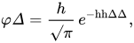
Although Gauss was the first to suggest the normal distribution law, Laplace made significant contributions.[note 4] It was Laplace who first posed the problem of aggregating several observations in 1774,[71] although his own solution led to the Laplacian distribution. It was Laplace who first calculated the value of the integral ∫ e−t2 dt = √π in 1782, providing the normalization constant for the normal distribution.[72] Finally, it was Laplace who in 1810 proved and presented to the academy the fundamental central limit theorem, which emphasized the theoretical importance of the normal distribution.[73]
It is of interest to note that in 1809 an Irish-American mathematician Robert Adrain published two insightful but flawed derivations of the normal probability law, simultaneously and independently from Gauss.[74] His works remained largely unnoticed by the scientific community, until in 1871 they were exhumed by Abbe.[75]
In the middle of the 19th century Maxwell demonstrated that the normal distribution is not just a convenient mathematical tool, but may also occur in natural phenomena:[76] The number of particles whose velocity, resolved in a certain direction, lies between x and x + dx is
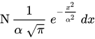
Naming
Today, the concept is usually known in English as the normal distribution or Gaussian distribution. Other less common names include Gauss distribution, Laplace-Gauss distribution, the law of error, the law of facility of errors, Laplace's second law, and Gaussian law.
Gauss himself apparently coined the term with reference to the "normal equations" involved in its applications, with normal having its technical meaning of orthogonal rather than usual.[77] However, by the end of the 19th century some authors[note 5] had started using the name normal distribution, where the word "normal" was used as an adjective – the term now being seen as a reflection of the fact that this distribution was seen as typical, common – and thus normal. Peirce (one of those authors) once defined "normal" thus: "...the 'normal' is not the average (or any other kind of mean) of what actually occurs, but of what would, in the long run, occur under certain circumstances."[78] Around the turn of the 20th century Pearson popularized the term normal as a designation for this distribution.[79]
Many years ago I called the Laplace–Gaussian curve the normal curve, which name, while it avoids an international question of priority, has the disadvantage of leading people to believe that all other distributions of frequency are in one sense or another 'abnormal'.
— Pearson (1920)
Also, it was Pearson who first wrote the distribution in terms of the standard deviation σ as in modern notation. Soon after this, in year 1915, Fisher added the location parameter to the formula for normal distribution, expressing it in the way it is written nowadays:
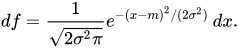
The term "standard normal", which denotes the normal distribution with zero mean and unit variance came into general use around the 1950s, appearing in the popular textbooks by P. G. Hoel (1947) Introduction to Mathematical Statistics and A. M. Mood (1950) Introduction to the Theory of Statistics.[80]
See also

- Bates distribution – similar to the Irwin–Hall distribution, but rescaled back into the 0 to 1 range
- Behrens–Fisher problem – the long-standing problem of testing whether two normal samples with different variances have same means;
- Bhattacharyya distance – method used to separate mixtures of normal distributions
- Erdős–Kac theorem – on the occurrence of the normal distribution in number theory
- Full width at half maximum
- Gaussian blur – convolution, which uses the normal distribution as a kernel
- Modified half-normal distribution[81] with the pdf on is given as , where denotes the Fox–Wright Psi function.
- Normally distributed and uncorrelated does not imply independent
- Ratio normal distribution
- Reciprocal normal distribution
- Standard normal table
- Stein's lemma
- Sub-Gaussian distribution
- Sum of normally distributed random variables
- Tweedie distribution – The normal distribution is a member of the family of Tweedie exponential dispersion models.
- Wrapped normal distribution – the Normal distribution applied to a circular domain
- Z-test – using the normal distribution


Notes
- ^ For example, this algorithm is given in the article Bc programming language.
- ^ De Moivre first published his findings in 1733, in a pamphlet Approximatio ad Summam Terminorum Binomii (a + b)n in Seriem Expansi that was designated for private circulation only. But it was not until the year 1738 that he made his results publicly available. The original pamphlet was reprinted several times, see for example Walker (1985).
- ^ "It has been customary certainly to regard as an axiom the hypothesis that if any quantity has been determined by several direct observations, made under the same circumstances and with equal care, the arithmetical mean of the observed values affords the most probable value, if not rigorously, yet very nearly at least, so that it is always most safe to adhere to it." — Gauss (1809, section 177)
- ^ "My custom of terming the curve the Gauss–Laplacian or normal curve saves us from proportioning the merit of discovery between the two great astronomer mathematicians." quote from Pearson (1905, p. 189)
- ^ Besides those specifically referenced here, such use is encountered in the works of Peirce, Galton (Galton (1889, chapter V)) and Lexis (Lexis (1878), Rohrbasser & Véron (2003)) c. 1875.[citation needed]
References
Citations
- ^ Norton, Matthew; Khokhlov, Valentyn; Uryasev, Stan (2019). "Calculating CVaR and bPOE for common probability distributions with application to portfolio optimization and density estimation" (PDF). Annals of Operations Research. 299 (1–2). Springer: 1281–1315. arXiv:1811.11301. doi:10.1007/s10479-019-03373-1. S2CID 254231768. Retrieved February 27, 2023.
- ^ Normal Distribution, Gale Encyclopedia of Psychology
- ^ Casella & Berger (2001, p. 102)
- ^ Lyon, A. (2014). Why are Normal Distributions Normal?, The British Journal for the Philosophy of Science.
- ^ Jorge, Nocedal; Stephan, J. Wright (2006). Numerical Optimization (2nd ed.). Springer. p. 249. ISBN 978-0387-30303-1.
- ^ a b "Normal Distribution". www.mathsisfun.com. Retrieved August 15, 2020.
- ^ Stigler (1982)
- ^ Halperin, Hartley & Hoel (1965, item 7)
- ^ McPherson (1990, p. 110)
- ^ Bernardo & Smith (2000, p. 121)
- ^ Scott, Clayton; Nowak, Robert (August 7, 2003). "The Q-function". Connexions.
- ^ Barak, Ohad (April 6, 2006). "Q Function and Error Function" (PDF). Tel Aviv University. Archived from the original (PDF) on March 25, 2009.
- ^ Weisstein, Eric W. "Normal Distribution Function". MathWorld.
- ^ Abramowitz, Milton; Stegun, Irene Ann, eds. (1983) [June 1964]. "Chapter 26, eqn 26.2.12". Handbook of Mathematical Functions with Formulas, Graphs, and Mathematical Tables. Applied Mathematics Series. Vol. 55 (Ninth reprint with additional corrections of tenth original printing with corrections (December 1972); first ed.). Washington D.C.; New York: United States Department of Commerce, National Bureau of Standards; Dover Publications. p. 932. ISBN 978-0-486-61272-0. LCCN 64-60036. MR 0167642. LCCN 65-12253.
- ^ Vaart, A. W. van der (October 13, 1998). Asymptotic Statistics. Cambridge University Press. doi:10.1017/cbo9780511802256. ISBN 978-0-511-80225-6.
- ^ Cover, Thomas M.; Thomas, Joy A. (2006). Elements of Information Theory. John Wiley and Sons. p. 254. ISBN 9780471748816.
- ^ Park, Sung Y.; Bera, Anil K. (2009). "Maximum Entropy Autoregressive Conditional Heteroskedasticity Model" (PDF). Journal of Econometrics. 150 (2): 219–230. CiteSeerX 10.1.1.511.9750. doi:10.1016/j.jeconom.2008.12.014. Archived from the original (PDF) on March 7, 2016. Retrieved June 2, 2011.
- ^ Geary RC(1936) The distribution of the "Student's ratio for the non-normal samples". Supplement to the Journal of the Royal Statistical Society 3 (2): 178–184
- ^ Lukacs, Eugene (March 1942). "A Characterization of the Normal Distribution". Annals of Mathematical Statistics. 13 (1): 91–93. doi:10.1214/AOMS/1177731647. ISSN 0003-4851. JSTOR 2236166. MR 0006626. Zbl 0060.28509. Wikidata Q55897617.
- ^ a b c Patel & Read (1996, [2.1.4])
- ^ Fan (1991, p. 1258)
- ^ Patel & Read (1996, [2.1.8])
- ^ Papoulis, Athanasios. Probability, Random Variables and Stochastic Processes (4th ed.). p. 148.
- ^ Winkelbauer, Andreas (2012). "Moments and Absolute Moments of the Normal Distribution". arXiv:1209.4340 [math.ST].
- ^ Bryc (1995, p. 23)
- ^ Bryc (1995, p. 24)
- ^ Cover & Thomas (2006, p. 254)
- ^ Williams, David (2001). Weighing the odds : a course in probability and statistics (Reprinted. ed.). Cambridge [u.a.]: Cambridge Univ. Press. pp. 197–199. ISBN 978-0-521-00618-7.
- ^ Smith, José M. Bernardo; Adrian F. M. (2000). Bayesian theory (Reprint ed.). Chichester [u.a.]: Wiley. pp. 209, 366. ISBN 978-0-471-49464-5.
{{cite book}}: CS1 maint: multiple names: authors list (link) - ^ O'Hagan, A. (1994) Kendall's Advanced Theory of statistics, Vol 2B, Bayesian Inference, Edward Arnold. ISBN 0-340-52922-9 (Section 5.40)
- ^ a b Bryc (1995, p. 35)
- ^ UIUC, Lecture 21. The Multivariate Normal Distribution, 21.6:"Individually Gaussian Versus Jointly Gaussian".
- ^ Edward L. Melnick and Aaron Tenenbein, "Misspecifications of the Normal Distribution", The American Statistician, volume 36, number 4 November 1982, pages 372–373
- ^ "Kullback Leibler (KL) Distance of Two Normal (Gaussian) Probability Distributions". Allisons.org. December 5, 2007. Retrieved March 3, 2017.
- ^ Jordan, Michael I. (February 8, 2010). "Stat260: Bayesian Modeling and Inference: The Conjugate Prior for the Normal Distribution" (PDF).
- ^ Amari & Nagaoka (2000)
- ^ "Expectation of the maximum of gaussian random variables". Mathematics Stack Exchange. Retrieved April 7, 2024.
- ^ "Normal Approximation to Poisson Distribution". Stat.ucla.edu. Retrieved March 3, 2017.
- ^ a b Das, Abhranil (2021). "A method to integrate and classify normal distributions". Journal of Vision. 21 (10): 1. arXiv:2012.14331. doi:10.1167/jov.21.10.1. PMC 8419883. PMID 34468706.
- ^ Bryc (1995, p. 27)
- ^ Weisstein, Eric W. "Normal Product Distribution". MathWorld. wolfram.com.
- ^ Lukacs, Eugene (1942). "A Characterization of the Normal Distribution". The Annals of Mathematical Statistics. 13 (1): 91–3. doi:10.1214/aoms/1177731647. ISSN 0003-4851. JSTOR 2236166.
- ^ Basu, D.; Laha, R. G. (1954). "On Some Characterizations of the Normal Distribution". Sankhyā. 13 (4): 359–62. ISSN 0036-4452. JSTOR 25048183.
- ^ Lehmann, E. L. (1997). Testing Statistical Hypotheses (2nd ed.). Springer. p. 199. ISBN 978-0-387-94919-2.
- ^ Patel & Read (1996, [2.3.6])
- ^ Galambos & Simonelli (2004, Theorem 3.5)
- ^ a b Lukacs & King (1954)
- ^ Quine, M.P. (1993). "On three characterisations of the normal distribution". Probability and Mathematical Statistics. 14 (2): 257–263.
- ^ John, S (1982). "The three parameter two-piece normal family of distributions and its fitting". Communications in Statistics – Theory and Methods. 11 (8): 879–885. doi:10.1080/03610928208828279.
- ^ a b Krishnamoorthy (2006, p. 127)
- ^ Krishnamoorthy (2006, p. 130)
- ^ Krishnamoorthy (2006, p. 133)
- ^ Huxley (1932)
- ^ Jaynes, Edwin T. (2003). Probability Theory: The Logic of Science. Cambridge University Press. pp. 592–593. ISBN 9780521592710.
- ^ Oosterbaan, Roland J. (1994). "Chapter 6: Frequency and Regression Analysis of Hydrologic Data" (PDF). In Ritzema, Henk P. (ed.). Drainage Principles and Applications, Publication 16 (second revised ed.). Wageningen, The Netherlands: International Institute for Land Reclamation and Improvement (ILRI). pp. 175–224. ISBN 978-90-70754-33-4.
- ^ Why Most Published Research Findings Are False, John P. A. Ioannidis, 2005
- ^ Wichura, Michael J. (1988). "Algorithm AS241: The Percentage Points of the Normal Distribution". Applied Statistics. 37 (3): 477–84. doi:10.2307/2347330. JSTOR 2347330.
- ^ Johnson, Kotz & Balakrishnan (1995, Equation (26.48))
- ^ Kinderman & Monahan (1977)
- ^ Leva (1992)
- ^ Marsaglia & Tsang (2000)
- ^ Karney (2016)
- ^ Monahan (1985, section 2)
- ^ Wallace (1996)
- ^ Johnson, Kotz & Balakrishnan (1994, p. 85)
- ^ Le Cam & Lo Yang (2000, p. 74)
- ^ De Moivre, Abraham (1733), Corollary I – see Walker (1985, p. 77)
- ^ Stigler (1986, p. 76)
- ^ Gauss (1809, section 177)
- ^ Gauss (1809, section 179)
- ^ Laplace (1774, Problem III)
- ^ Pearson (1905, p. 189)
- ^ Stigler (1986, p. 144)
- ^ Stigler (1978, p. 243)
- ^ Stigler (1978, p. 244)
- ^ Maxwell (1860, p. 23)
- ^ Jaynes, Edwin J.; Probability Theory: The Logic of Science, Ch. 7.
- ^ Peirce, Charles S. (c. 1909 MS), Collected Papers v. 6, paragraph 327.
- ^ Kruskal & Stigler (1997).
- ^ "Earliest Uses... (Entry Standard Normal Curve)".
- ^ Sun, Jingchao; Kong, Maiying; Pal, Subhadip (June 22, 2021). "The Modified-Half-Normal distribution: Properties and an efficient sampling scheme". Communications in Statistics – Theory and Methods. 52 (5): 1591–1613. doi:10.1080/03610926.2021.1934700. ISSN 0361-0926. S2CID 237919587.
Sources
- Aldrich, John; Miller, Jeff. "Earliest Uses of Symbols in Probability and Statistics".
- Aldrich, John; Miller, Jeff. "Earliest Known Uses of Some of the Words of Mathematics". In particular, the entries for "bell-shaped and bell curve", "normal (distribution)", "Gaussian", and "Error, law of error, theory of errors, etc.".
- Amari, Shun-ichi; Nagaoka, Hiroshi (2000). Methods of Information Geometry. Oxford University Press. ISBN 978-0-8218-0531-2.
- Bernardo, José M.; Smith, Adrian F. M. (2000). Bayesian Theory. Wiley. ISBN 978-0-471-49464-5.
- Bryc, Wlodzimierz (1995). The Normal Distribution: Characterizations with Applications. Springer-Verlag. ISBN 978-0-387-97990-8.
- Casella, George; Berger, Roger L. (2001). Statistical Inference (2nd ed.). Duxbury. ISBN 978-0-534-24312-8.
- Cody, William J. (1969). "Rational Chebyshev Approximations for the Error Function". Mathematics of Computation. 23 (107): 631–638. doi:10.1090/S0025-5718-1969-0247736-4.
- Cover, Thomas M.; Thomas, Joy A. (2006). Elements of Information Theory. John Wiley and Sons.
- Dia, Yaya D. (2023). "Approximate Incomplete Integrals, Application to Complementary Error Function". SSRN. doi:10.2139/ssrn.4487559. S2CID 259689086.
- de Moivre, Abraham (1738). The Doctrine of Chances. American Mathematical Society. ISBN 978-0-8218-2103-9.
- Fan, Jianqing (1991). "On the optimal rates of convergence for nonparametric deconvolution problems". The Annals of Statistics. 19 (3): 1257–1272. doi:10.1214/aos/1176348248. JSTOR 2241949.
- Galton, Francis (1889). Natural Inheritance (PDF). London, UK: Richard Clay and Sons.
- Galambos, Janos; Simonelli, Italo (2004). Products of Random Variables: Applications to Problems of Physics and to Arithmetical Functions. Marcel Dekker, Inc. ISBN 978-0-8247-5402-0.
- Gauss, Carolo Friderico (1809). Theoria motvs corporvm coelestivm in sectionibvs conicis Solem ambientivm [Theory of the Motion of the Heavenly Bodies Moving about the Sun in Conic Sections] (in Latin). Hambvrgi, Svmtibvs F. Perthes et I. H. Besser. English translation.
- Gould, Stephen Jay (1981). The Mismeasure of Man (first ed.). W. W. Norton. ISBN 978-0-393-01489-1.
- Halperin, Max; Hartley, Herman O.; Hoel, Paul G. (1965). "Recommended Standards for Statistical Symbols and Notation. COPSS Committee on Symbols and Notation". The American Statistician. 19 (3): 12–14. doi:10.2307/2681417. JSTOR 2681417.
- Hart, John F.; et al. (1968). Computer Approximations. New York, NY: John Wiley & Sons, Inc. ISBN 978-0-88275-642-4.
- "Normal Distribution", Encyclopedia of Mathematics, EMS Press, 2001 [1994]
- Herrnstein, Richard J.; Murray, Charles (1994). The Bell Curve: Intelligence and Class Structure in American Life. Free Press. ISBN 978-0-02-914673-6.
- Huxley, Julian S. (1932). Problems of Relative Growth. London. ISBN 978-0-486-61114-3. OCLC 476909537.
- Johnson, Norman L.; Kotz, Samuel; Balakrishnan, Narayanaswamy (1994). Continuous Univariate Distributions, Volume 1. Wiley. ISBN 978-0-471-58495-7.
- Johnson, Norman L.; Kotz, Samuel; Balakrishnan, Narayanaswamy (1995). Continuous Univariate Distributions, Volume 2. Wiley. ISBN 978-0-471-58494-0.
- Karney, C. F. F. (2016). "Sampling exactly from the normal distribution". ACM Transactions on Mathematical Software. 42 (1): 3:1–14. arXiv:1303.6257. doi:10.1145/2710016. S2CID 14252035.
- Kinderman, Albert J.; Monahan, John F. (1977). "Computer Generation of Random Variables Using the Ratio of Uniform Deviates". ACM Transactions on Mathematical Software. 3 (3): 257–260. doi:10.1145/355744.355750. S2CID 12884505.
- Krishnamoorthy, Kalimuthu (2006). Handbook of Statistical Distributions with Applications. Chapman & Hall/CRC. ISBN 978-1-58488-635-8.
- Kruskal, William H.; Stigler, Stephen M. (1997). Spencer, Bruce D. (ed.). Normative Terminology: 'Normal' in Statistics and Elsewhere. Statistics and Public Policy. Oxford University Press. ISBN 978-0-19-852341-3.
- Laplace, Pierre-Simon de (1774). "Mémoire sur la probabilité des causes par les événements". Mémoires de l'Académie Royale des Sciences de Paris (Savants étrangers), Tome 6: 621–656. Translated by Stephen M. Stigler in Statistical Science 1 (3), 1986: JSTOR 2245476.
- Laplace, Pierre-Simon (1812). Théorie analytique des probabilités [Analytical theory of probabilities]. Paris, Ve. Courcier.
- Le Cam, Lucien; Lo Yang, Grace (2000). Asymptotics in Statistics: Some Basic Concepts (second ed.). Springer. ISBN 978-0-387-95036-5.
- Leva, Joseph L. (1992). "A fast normal random number generator" (PDF). ACM Transactions on Mathematical Software. 18 (4): 449–453. CiteSeerX 10.1.1.544.5806. doi:10.1145/138351.138364. S2CID 15802663. Archived from the original (PDF) on July 16, 2010.
- Lexis, Wilhelm (1878). "Sur la durée normale de la vie humaine et sur la théorie de la stabilité des rapports statistiques". Annales de Démographie Internationale. II. Paris: 447–462.
- Lukacs, Eugene; King, Edgar P. (1954). "A Property of Normal Distribution". The Annals of Mathematical Statistics. 25 (2): 389–394. doi:10.1214/aoms/1177728796. JSTOR 2236741.
- McPherson, Glen (1990). Statistics in Scientific Investigation: Its Basis, Application and Interpretation. Springer-Verlag. ISBN 978-0-387-97137-7.
- Marsaglia, George; Tsang, Wai Wan (2000). "The Ziggurat Method for Generating Random Variables". Journal of Statistical Software. 5 (8). doi:10.18637/jss.v005.i08.
- Marsaglia, George (2004). "Evaluating the Normal Distribution". Journal of Statistical Software. 11 (4). doi:10.18637/jss.v011.i04.
- Maxwell, James Clerk (1860). "V. Illustrations of the dynamical theory of gases. — Part I: On the motions and collisions of perfectly elastic spheres". Philosophical Magazine. Series 4. 19 (124): 19–32. doi:10.1080/14786446008642818.
- Monahan, J. F. (1985). "Accuracy in random number generation". Mathematics of Computation. 45 (172): 559–568. doi:10.1090/S0025-5718-1985-0804945-X.
- Patel, Jagdish K.; Read, Campbell B. (1996). Handbook of the Normal Distribution (2nd ed.). CRC Press. ISBN 978-0-8247-9342-5.
- Pearson, Karl (1901). "On Lines and Planes of Closest Fit to Systems of Points in Space" (PDF). Philosophical Magazine. 6. 2 (11): 559–572. doi:10.1080/14786440109462720. S2CID 125037489.
- Pearson, Karl (1905). "'Das Fehlergesetz und seine Verallgemeinerungen durch Fechner und Pearson'. A rejoinder". Biometrika. 4 (1): 169–212. doi:10.2307/2331536. JSTOR 2331536.
- Pearson, Karl (1920). "Notes on the History of Correlation". Biometrika. 13 (1): 25–45. doi:10.1093/biomet/13.1.25. JSTOR 2331722.
- Rohrbasser, Jean-Marc; Véron, Jacques (2003). "Wilhelm Lexis: The Normal Length of Life as an Expression of the "Nature of Things"". Population. 58 (3): 303–322. doi:10.3917/pope.303.0303.
- Shore, H (1982). "Simple Approximations for the Inverse Cumulative Function, the Density Function and the Loss Integral of the Normal Distribution". Journal of the Royal Statistical Society. Series C (Applied Statistics). 31 (2): 108–114. doi:10.2307/2347972. JSTOR 2347972.
- Shore, H (2005). "Accurate RMM-Based Approximations for the CDF of the Normal Distribution". Communications in Statistics – Theory and Methods. 34 (3): 507–513. doi:10.1081/sta-200052102. S2CID 122148043.
- Shore, H (2011). "Response Modeling Methodology". WIREs Comput Stat. 3 (4): 357–372. doi:10.1002/wics.151. S2CID 62021374.
- Shore, H (2012). "Estimating Response Modeling Methodology Models". WIREs Comput Stat. 4 (3): 323–333. doi:10.1002/wics.1199. S2CID 122366147.
- Stigler, Stephen M. (1978). "Mathematical Statistics in the Early States". The Annals of Statistics. 6 (2): 239–265. doi:10.1214/aos/1176344123. JSTOR 2958876.
- Stigler, Stephen M. (1982). "A Modest Proposal: A New Standard for the Normal". The American Statistician. 36 (2): 137–138. doi:10.2307/2684031. JSTOR 2684031.
- Stigler, Stephen M. (1986). The History of Statistics: The Measurement of Uncertainty before 1900. Harvard University Press. ISBN 978-0-674-40340-6.
- Stigler, Stephen M. (1999). Statistics on the Table. Harvard University Press. ISBN 978-0-674-83601-3.
- Walker, Helen M. (1985). "De Moivre on the Law of Normal Probability" (PDF). In Smith, David Eugene (ed.). A Source Book in Mathematics. Dover. ISBN 978-0-486-64690-9.
- Wallace, C. S. (1996). "Fast pseudo-random generators for normal and exponential variates". ACM Transactions on Mathematical Software. 22 (1): 119–127. doi:10.1145/225545.225554. S2CID 18514848.
- Weisstein, Eric W. "Normal Distribution". MathWorld.
- West, Graeme (2009). "Better Approximations to Cumulative Normal Functions" (PDF). Wilmott Magazine: 70–76. Archived from the original (PDF) on February 29, 2012.
- Zelen, Marvin; Severo, Norman C. (1964). Probability Functions (chapter 26). Handbook of mathematical functions with formulas, graphs, and mathematical tables, by Abramowitz, M.; and Stegun, I. A.: National Bureau of Standards. New York, NY: Dover. ISBN 978-0-486-61272-0.
External links

- "Normal distribution", Encyclopedia of Mathematics, EMS Press, 2001 [1994]
- Normal distribution calculator


