Articulo de referencia

Lista de transformaciones de coordenadas comunes

Esta es una lista de algunas de las transformaciones de coordenadas más comúnmente utilizadas . Bidimensional Sean las coordenadas cartesianas estándar y las coordenadas polares...

Esta es una lista de algunas de las transformaciones de coordenadas más comúnmente utilizadas .

Bidimensional

Sean las coordenadas cartesianas estándar y las coordenadas polares estándar . ( incógnita , y ) {\estilo de visualización (x,y)} ( a , θ ) {\displaystyle (r,\theta )}

A coordenadas cartesianas

Desde coordenadas polares

incógnita = a porque θ y = a pecado θ ( incógnita , y ) ( a , θ ) = [ porque θ a pecado θ pecado θ a porque θ ] Jacobiano = det ( incógnita , y ) ( a , θ ) = a {\displaystyle {\begin{aligned}x&=r\cos \theta \\y&=r\sin \theta \\[5pt]{\frac {\partial (x,y)}{\partial (r,\theta )}}&={\begin{bmatrix}\cos \theta &-r\sin \theta \\\sin \theta &{\phantom {-}}r\cos \theta \end{bmatrix}}\\[5pt]{\text{Jacobian}}=\det {\frac {\partial (x,y)}{\partial (r,\theta )}}&=r\end{aligned}}}

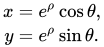
A partir de coordenadas log-polares

x = e ρ cos θ , y = e ρ sin θ . {\displaystyle {\begin{aligned}x&=e^{\rho }\cos \theta ,\\y&=e^{\rho }\sin \theta .\end{aligned}}}

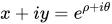
Usando números complejos , la transformación se puede escribir como ( x , y ) = x + i y {\displaystyle (x,y)=x+iy'} x + i y = e ρ + i θ {\displaystyle x+iy=e^{\rho +i\theta }}

Es decir, viene dada por la función exponencial compleja.

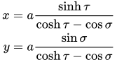
Desde coordenadas bipolares

x = a sinh τ cosh τ cos σ y = a sin σ cosh τ cos σ {\displaystyle {\begin{aligned}x&=a{\frac {\sinh \tau }{\cosh \tau -\cos \sigma }}\\y&=a{\frac {\sin \sigma }{\cosh \tau -\cos \sigma }}\end{aligned}}}

A partir de coordenadas bipolares de 2 centros

x = 1 4 c ( r 1 2 r 2 2 ) y = ± 1 4 c 16 c 2 r 1 2 ( r 1 2 r 2 2 + 4 c 2 ) 2 {\displaystyle {\begin{aligned}x&={\frac {1}{4c}}\left(r_{1}^{2}-r_{2}^{2}\right)\\[1ex]y&=\pm {\frac {1}{4c}}{\sqrt {16c^{2}r_{1}^{2}-\left(r_{1}^{2}-r_{2}^{2}+4c^{2}\right)^{2}}}\end{aligned}}}

De la ecuación de Cesáro

x = cos [ κ ( s ) d s ] d s y = sin [ κ ( s ) d s ] d s {\displaystyle {\begin{aligned}x&=\int \cos \left[\int \kappa (s)\,ds\right]ds\\y&=\int \sin \left[\int \kappa (s)\,ds\right]ds\end{aligned}}}

A coordenadas polares

Desde coordenadas cartesianas

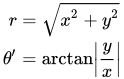
r = x 2 + y 2 θ = arctan | y x | {\displaystyle {\begin{aligned}r&={\sqrt {x^{2}+y^{2}}}\\\theta '&=\arctan \left|{\frac {y}{x}}\right|\end{aligned}}} Nota: al resolver para se obtiene el ángulo resultante en el primer cuadrante ( ). Para hallarlo, hay que recurrir a la coordenada cartesiana original, determinar el cuadrante en el que se encuentra (por ejemplo, (3,−3) [cartesiana] se encuentra en QIV), y luego utilizar lo siguiente para resolver θ {\displaystyle \theta '} 0 < θ < π 2 {\textstyle 0<\theta <{\frac {\pi }{2}}} θ , {\displaystyle \theta ,} θ {\displaystyle \theta } θ : {\displaystyle \theta :}

θ = { θ for  θ  in QI:  0 < θ < π 2 π θ for  θ  in QII:  π 2 < θ < π π + θ for  θ  in QIII:  π < θ < 3 π 2 2 π θ for  θ  in QIV:  3 π 2 < θ < 2 π {\displaystyle \theta ={\begin{cases}\theta '&{\text{for }}\theta '{\text{ in QI: }}&0<\theta '<{\frac {\pi }{2}}\\[1.2ex]\pi -\theta '&{\text{for }}\theta '{\text{ in QII: }}&{\frac {\pi }{2}}<\theta '<\pi \\[1.2ex]\pi +\theta '&{\text{for }}\theta '{\text{ in QIII: }}&\pi <\theta '<{\frac {3\pi }{2}}\\[1.2ex]2\pi -\theta '&{\text{for }}\theta '{\text{ in QIV: }}&{\frac {3\pi }{2}}<\theta '<2\pi \end{cases}}}

El valor de se debe resolver de esta manera porque para todos los valores de , solo está definido para , y es periódico (con período ). Esto significa que la función inversa solo dará valores en el dominio de la función, pero restringidos a un solo período. Por lo tanto, el rango de la función inversa es solo la mitad de un círculo completo. θ {\displaystyle \theta } θ {\displaystyle \theta } tan θ {\displaystyle \tan \theta } π 2 < θ < + π 2 {\textstyle -{\frac {\pi }{2}}<\theta <+{\frac {\pi }{2}}} π {\displaystyle \pi }

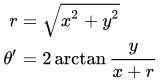
Tenga en cuenta que también se puede utilizar r = x 2 + y 2 θ = 2 arctan y x + r {\displaystyle {\begin{aligned}r&={\sqrt {x^{2}+y^{2}}}\\\theta '&=2\arctan {\frac {y}{x+r}}\end{aligned}}}

A partir de coordenadas bipolares de 2 centros

r = r 1 2 + r 2 2 2 c 2 2 θ = arctan [ 8 c 2 ( r 1 2 + r 2 2 2 c 2 ) r 1 2 r 2 2 1 ] {\displaystyle {\begin{aligned}r&={\sqrt {\frac {r_{1}^{2}+r_{2}^{2}-2c^{2}}{2}}}\\\theta &=\arctan \left[{\sqrt {{\frac {8c^{2}(r_{1}^{2}+r_{2}^{2}-2c^{2})}{r_{1}^{2}-r_{2}^{2}}}-1}}\right]\end{aligned}}}

Donde 2 c es la distancia entre los polos.

Para coordenadas logarítmicas polares a partir de coordenadas cartesianas

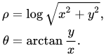
ρ = log x 2 + y 2 , θ = arctan y x . {\displaystyle {\begin{aligned}\rho &=\log {\sqrt {x^{2}+y^{2}}},\\\theta &=\arctan {\frac {y}{x}}.\end{aligned}}}

Longitud de arco y curvatura

En coordenadas cartesianas

κ = x y y x ( x 2 + y 2 ) 3 2 s = a t x 2 + y 2 d t {\displaystyle {\begin{aligned}\kappa &={\frac {x'y''-y'x''}{\left({x'}^{2}+{y'}^{2}\right)^{\frac {3}{2}}}}\\s&=\int _{a}^{t}{\sqrt {{x'}^{2}+{y'}^{2}}}\,dt\end{aligned}}}

En coordenadas polares

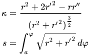
κ = r 2 + 2 r 2 r r ( r 2 + r 2 ) 3 2 s = a φ r 2 + r 2 d φ {\displaystyle {\begin{aligned}\kappa &={\frac {r^{2}+2{r'}^{2}-rr''}{(r^{2}+{r'}^{2})^{\frac {3}{2}}}}\\s&=\int _{a}^{\varphi }{\sqrt {r^{2}+{r'}^{2}}}\,d\varphi \end{aligned}}}

3-dimensional

Sean (x, y, z) las coordenadas cartesianas estándar y (ρ, θ, φ) las coordenadas esféricas , con θ el ángulo medido a partir del eje +Z (como [1], véanse las convenciones en coordenadas esféricas ). Como φ tiene un rango de 360°, se aplican las mismas consideraciones que en las coordenadas polares (bidimensionales) siempre que se tome un arcotangente de este. θ tiene un rango de 180°, que va de 0° a 180°, y no plantea ningún problema cuando se calcula a partir de un arcocoseno, pero tenga cuidado con un arcotangente.

Si, en la definición alternativa, se elige que θ se extienda de −90° a +90°, en dirección opuesta a la definición anterior, se puede hallar únicamente a partir de un arcoseno, pero hay que tener cuidado con un arcocotangente. En este caso, en todas las fórmulas que aparecen a continuación, todos los argumentos de θ deben tener seno y coseno intercambiados, y como derivada también un más y un menos intercambiados.

Todas las divisiones por cero resultan en casos especiales de ser direcciones a lo largo de uno de los ejes principales y en la práctica se resuelven más fácilmente mediante la observación.

A coordenadas cartesianas

A partir de coordenadas esféricas

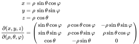
x = ρ sin θ cos φ y = ρ sin θ sin φ z = ρ cos θ ( x , y , z ) ( ρ , θ , φ ) = ( sin θ cos φ ρ cos θ cos φ ρ sin θ sin φ sin θ sin φ ρ cos θ sin φ ρ sin θ cos φ cos θ ρ sin θ 0 ) {\displaystyle {\begin{aligned}x&=\rho \,\sin \theta \cos \varphi \\y&=\rho \,\sin \theta \sin \varphi \\z&=\rho \,\cos \theta \\{\frac {\partial (x,y,z)}{\partial (\rho ,\theta ,\varphi )}}&={\begin{pmatrix}\sin \theta \cos \varphi &\rho \cos \theta \cos \varphi &-\rho \sin \theta \sin \varphi \\\sin \theta \sin \varphi &\rho \cos \theta \sin \varphi &\rho \sin \theta \cos \varphi \\\cos \theta &-\rho \sin \theta &0\end{pmatrix}}\end{aligned}}}

Entonces, para el elemento de volumen: d x d y d z = det ( x , y , z ) ( ρ , θ , φ ) d ρ d θ d φ = ρ 2 sin θ d ρ d θ d φ {\displaystyle dx\,dy\,dz=\det {\frac {\partial (x,y,z)}{\partial (\rho ,\theta ,\varphi )}}\,d\rho \,d\theta \,d\varphi =\rho ^{2}\sin \theta \,d\rho \,d\theta \,d\varphi }

A partir de coordenadas cilíndricas

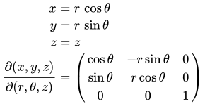
x = r cos θ y = r sin θ z = z ( x , y , z ) ( r , θ , z ) = ( cos θ r sin θ 0 sin θ r cos θ 0 0 0 1 ) {\displaystyle {\begin{aligned}x&=r\,\cos \theta \\y&=r\,\sin \theta \\z&=z\,\\{\frac {\partial (x,y,z)}{\partial (r,\theta ,z)}}&={\begin{pmatrix}\cos \theta &-r\sin \theta &0\\\sin \theta &r\cos \theta &0\\0&0&1\end{pmatrix}}\end{aligned}}}

Entonces, para el elemento de volumen: d V = d x d y d z = det ( x , y , z ) ( r , θ , z ) d r d θ d z = r d r d θ d z {\displaystyle dV=dx\,dy\,dz=\det {\frac {\partial (x,y,z)}{\partial (r,\theta ,z)}}\,dr\,d\theta \,dz=r\,dr\,d\theta \,dz}

A coordenadas esféricas

Desde coordenadas cartesianas

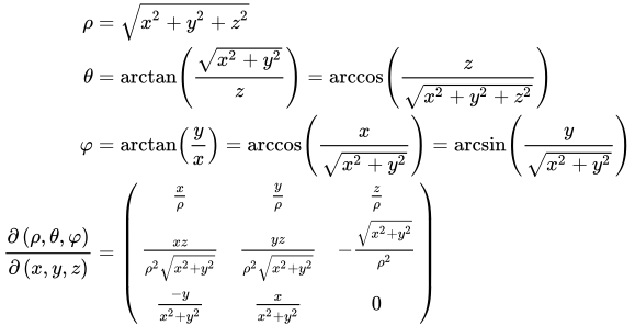
ρ = x 2 + y 2 + z 2 θ = arctan ( x 2 + y 2 z ) = arccos ( z x 2 + y 2 + z 2 ) φ = arctan ( y x ) = arccos ( x x 2 + y 2 ) = arcsin ( y x 2 + y 2 ) ( ρ , θ , φ ) ( x , y , z ) = ( x ρ y ρ z ρ x z ρ 2 x 2 + y 2 y z ρ 2 x 2 + y 2 x 2 + y 2 ρ 2 y x 2 + y 2 x x 2 + y 2 0 ) {\displaystyle {\begin{aligned}\rho &={\sqrt {x^{2}+y^{2}+z^{2}}}\\\theta &=\arctan \left({\frac {\sqrt {x^{2}+y^{2}}}{z}}\right)=\arccos \left({\frac {z}{\sqrt {x^{2}+y^{2}+z^{2}}}}\right)\\\varphi &=\arctan \left({\frac {y}{x}}\right)=\arccos \left({\frac {x}{\sqrt {x^{2}+y^{2}}}}\right)=\arcsin \left({\frac {y}{\sqrt {x^{2}+y^{2}}}}\right)\\{\frac {\partial \left(\rho ,\theta ,\varphi \right)}{\partial \left(x,y,z\right)}}&={\begin{pmatrix}{\frac {x}{\rho }}&{\frac {y}{\rho }}&{\frac {z}{\rho }}\\{\frac {xz}{\rho ^{2}{\sqrt {x^{2}+y^{2}}}}}&{\frac {yz}{\rho ^{2}{\sqrt {x^{2}+y^{2}}}}}&-{\frac {\sqrt {x^{2}+y^{2}}}{\rho ^{2}}}\\{\frac {-y}{x^{2}+y^{2}}}&{\frac {x}{x^{2}+y^{2}}}&0\\\end{pmatrix}}\end{aligned}}}

Consulte también el artículo sobre atan2 para saber cómo manejar con elegancia algunos casos extremos.

Entonces, para el elemento: d ρ d θ d φ = det ( ρ , θ , φ ) ( x , y , z ) d x d y d z = 1 x 2 + y 2 x 2 + y 2 + z 2 d x d y d z {\displaystyle d\rho \,d\theta \,d\varphi =\det {\frac {\partial (\rho ,\theta ,\varphi )}{\partial (x,y,z)}}\,dx\,dy\,dz={\frac {1}{{\sqrt {x^{2}+y^{2}}}{\sqrt {x^{2}+y^{2}+z^{2}}}}}\,dx\,dy\,dz}

A partir de coordenadas cilíndricas

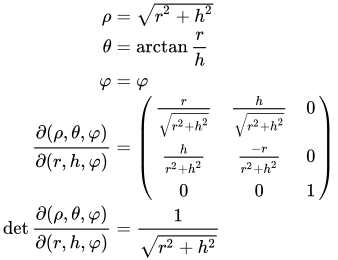
ρ = r 2 + h 2 θ = arctan r h φ = φ ( ρ , θ , φ ) ( r , h , φ ) = ( r r 2 + h 2 h r 2 + h 2 0 h r 2 + h 2 r r 2 + h 2 0 0 0 1 ) det ( ρ , θ , φ ) ( r , h , φ ) = 1 r 2 + h 2 {\displaystyle {\begin{aligned}\rho &={\sqrt {r^{2}+h^{2}}}\\\theta &=\arctan {\frac {r}{h}}\\\varphi &=\varphi \\{\frac {\partial (\rho ,\theta ,\varphi )}{\partial (r,h,\varphi )}}&={\begin{pmatrix}{\frac {r}{\sqrt {r^{2}+h^{2}}}}&{\frac {h}{\sqrt {r^{2}+h^{2}}}}&0\\{\frac {h}{r^{2}+h^{2}}}&{\frac {-r}{r^{2}+h^{2}}}&0\\0&0&1\\\end{pmatrix}}\\\det {\frac {\partial (\rho ,\theta ,\varphi )}{\partial (r,h,\varphi )}}&={\frac {1}{\sqrt {r^{2}+h^{2}}}}\end{aligned}}}

A coordenadas cilíndricas

Desde coordenadas cartesianas

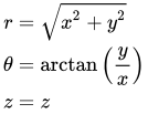
r = x 2 + y 2 θ = arctan ( y x ) z = z {\displaystyle {\begin{aligned}r&={\sqrt {x^{2}+y^{2}}}\\\theta &=\arctan {\left({\frac {y}{x}}\right)}\\z&=z\quad \end{aligned}}}

( r , θ , h ) ( x , y , z ) = ( x x 2 + y 2 y x 2 + y 2 0 y x 2 + y 2 x x 2 + y 2 0 0 0 1 ) {\displaystyle {\frac {\partial (r,\theta ,h)}{\partial (x,y,z)}}={\begin{pmatrix}{\frac {x}{\sqrt {x^{2}+y^{2}}}}&{\frac {y}{\sqrt {x^{2}+y^{2}}}}&0\\{\frac {-y}{x^{2}+y^{2}}}&{\frac {x}{x^{2}+y^{2}}}&0\\0&0&1\end{pmatrix}}}

A partir de coordenadas esféricas

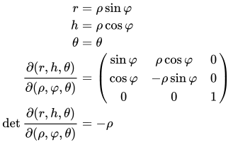
r = ρ sin φ h = ρ cos φ θ = θ ( r , h , θ ) ( ρ , φ , θ ) = ( sin φ ρ cos φ 0 cos φ ρ sin φ 0 0 0 1 ) det ( r , h , θ ) ( ρ , φ , θ ) = ρ {\displaystyle {\begin{aligned}r&=\rho \sin \varphi \\h&=\rho \cos \varphi \\\theta &=\theta \\{\frac {\partial (r,h,\theta )}{\partial (\rho ,\varphi ,\theta )}}&={\begin{pmatrix}\sin \varphi &\rho \cos \varphi &0\\\cos \varphi &-\rho \sin \varphi &0\\0&0&1\\\end{pmatrix}}\\\det {\frac {\partial (r,h,\theta )}{\partial (\rho ,\varphi ,\theta )}}&=-\rho \end{aligned}}}

Longitud de arco, curvatura y torsión a partir de coordenadas cartesianas

s = 0 t x 2 + y 2 + z 2 d t κ = ( z y y z ) 2 + ( x z z x ) 2 + ( y x x y ) 2 ( x 2 + y 2 + z 2 ) 3 2 τ = x ( y z y z ) + y ( x z x z ) + z ( x y x y ) ( x y x y ) 2 + ( x z x z ) 2 + ( y z y z ) 2 {\displaystyle {\begin{aligned}s&=\int _{0}^{t}{\sqrt {{x'}^{2}+{y'}^{2}+{z'}^{2}}}\,dt\\[3pt]\kappa &={\frac {\sqrt {\left(z''y'-y''z'\right)^{2}+\left(x''z'-z''x'\right)^{2}+\left(y''x'-x''y'\right)^{2}}}{\left({x'}^{2}+{y'}^{2}+{z'}^{2}\right)^{\frac {3}{2}}}}\\[3pt]\tau &={\frac {x'''\left(y'z''-y''z'\right)+y'''\left(x''z'-x'z''\right)+z'''\left(x'y''-x''y'\right)}{{\left(x'y''-x''y'\right)}^{2}+{\left(x''z'-x'z''\right)}^{2}+{\left(y'z''-y''z'\right)}^{2}}}\end{aligned}}}

Véase también

Referencias

  • Arfken, George (2013). Métodos matemáticos para físicos. Academic Press. ISBN 978-0123846549.
Retrieved from "https://en.wikipedia.org/w/index.php?title=List_of_common_coordinate_transformations&oldid=1251332927"