Núcleo (álgebra lineal)

Un ejemplo de núcleo: el operador lineal. $L:(x,y)\longrightarrow (x,x)$ transforma todos los puntos en el $(x=0,y)$ línea hasta el punto cero $(0,0)$ , por lo tanto, forman el núcleo del operador lineal

{\displaystyle L:(x,y)\longrightarrow (x,x)} — Un ejemplo de núcleo: el operador lineal. $L:(x,y)\longrightarrow (x,x)$ transforma todos los puntos en el $(x=0,y)$ línea hasta el punto cero $(0,0)$ , por lo tanto, forman el núcleo del operador lineal

En matemáticas , el núcleo de una aplicación lineal , también conocido como espacio nulo , es la parte del dominio que se mapea al vector cero del codominio ; el núcleo es siempre un subespacio lineal del dominio. ^[¹^] Es decir, dada una aplicación lineal $L$ $:$ $V$ $\to$ $W$ entre dos espacios vectoriales $V$ y $W$ , el núcleo de $L$ es el espacio vectorial de todos los elementos $v$ de $V$ tales que $L$ $($ $v$ $) =$ $0$ , donde $0$ denota el vector cero en $W$ , ^[²^] o de forma más simbólica: $\ker(L)=\left\{\mathbf {v} \in V\mid L(\mathbf {v} )=\mathbf {0} \right\}=L^{-1}(\mathbf {0} ).$

Propiedades

El núcleo de $L$ es un subespacio lineal del dominio $V.$ ^{[ 3 ]}^{[ 2 ]}

En el mapa lineal $L:V\to W,$ dos elementos de $V$ tienen la misma imagen en $W$ si y solo si su diferencia se encuentra en el núcleo de $L$ , es decir,

$L\left(\mathbf {v} _{1}\right)=L\left(\mathbf {v} _{2}\right)\quad \iff \quad L\left(\mathbf {v} _{1}-\mathbf {v} _{2}\right)=\mathbf {0} .$

De esto se deduce, por el primer teorema de isomorfismo , que la imagen de $L$ es isomorfa al cociente de $V$ por el núcleo: $\operatorname {im} (L)\cong V/\ker(L).$ En el caso en que $V$ sea de dimensión finita , esto implica el teorema de rango-nulidad : $\dim(\ker L)+\dim(\operatorname {im} L)=\dim(V).$ donde el términoEl rango se refiere a la dimensión de la imagen de $L$ , $\dim(\operatorname {estoy} L),$ mientrasLa nulidad se refiere a la dimensión del núcleo de $L$ , $\dim(\ker L).$ ^{[ 4 ]} Es decir, $\operatorname {Rango} (L)=\dim(\operatorname {im} L)\qquad {\text{ y }}\qquad \operatorname {Nulidad} (L)=\dim(\ker L),$ de modo que el teorema de rango-nulidad pueda reformularse como $\operatorname {Rango} (L)+\operatorname {Nulidad} (L)=\dim \left(\operatorname {dominio} L\right).$

Cuando $V$ es un espacio con producto interno , el cociente $V/\ker(L)$ puede identificarse con el complemento ortogonal en $V$ de $\ker(L)$ . Esta es la generalización a operadores lineales del espacio fila , o coimagen , de una matriz.

Generalización a módulos

La noción de núcleo también tiene sentido para los homomorfismos de módulos , que son generalizaciones de espacios vectoriales donde los escalares son elementos de un anillo , en lugar de un cuerpo . El dominio de la aplicación es un módulo, y el núcleo constituye un submódulo . En este caso, los conceptos de rango y nulidad no son necesariamente aplicables.

En el análisis funcional

Si $V$ y $W$ son espacios vectoriales topológicos tales que $W$ es de dimensión finita, entonces un operador lineal $L : V \to W$ es continuo si y solo si el núcleo de $L$ es un subespacio cerrado de $V.$

Representación como multiplicación de matrices

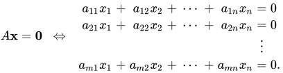
Consideremos un mapa lineal representado como una matriz $A$ $de m \times n$ con coeficientes en un campo $K$ (típicamente $\mathbb {R}$ o $\mathbb {C}$ ), es decir, operando sobre vectores columna $x$ con $n$ componentes sobre $K.$ El núcleo de esta aplicación lineal es el conjunto de soluciones de la ecuación $A x = 0$ , donde $0$ se entiende como el vector cero . La dimensión del núcleo de A se llama nulidad de A. En notación de constructor de conjuntos , $\operatorname {N} (A)=\operatorname {Null} (A)=\operatorname {ker} (A)=\left\{\mathbf {x} \in K^{n}\mid A\mathbf {x} =\mathbf {0} \right\}.$ La ecuación matricial es equivalente a un sistema homogéneo de ecuaciones lineales : $A\mathbf {x} =\mathbf {0} \;\;\Leftrightarrow \;\;{\begin{alignedat}{7}a_{11}x_{1}&&\;+\;&&a_{12}x_{2}&&\;+\;\cdots \;+\;&&a_{1n}x_{n}&&\;=\;&&&0\\a_{21}x_{1}&&\;+\;&&a_{22}x_{2}&&\;+\;\cdots \;+\;&&a_{2n}x_{n}&&\;=\;&&&0\\&&&&&&&&&&\vdots \ \;&&&\\a_{m1}x_{1}&&\;+\;&&a_{m2}x_{2}&&\;+\;\cdots \;+\;&&a_{mn}x_{n}&&\;=\;&&&0{\text{.}}\\\end{alignedat}}$ Por lo tanto, el núcleo de A es el mismo que el conjunto solución de las ecuaciones homogéneas anteriores.

Propiedades del subespacio

El núcleo de una matriz $m \times n$ $A$ sobre un cuerpo $K$ es un subespacio lineal de $K n$ . Es decir, el núcleo de $A$ , el conjunto $Null(A)$ , tiene las siguientes tres propiedades:

$Null(A)$ siempre contiene el vector cero , ya que $A 0 = 0$ .
Si $x \in Null(A)$ e $y \in Null(A)$ , entonces $x + y \in Null(A)$ . Esto se deduce de la propiedad distributiva de la multiplicación de matrices sobre la suma.
If $x \in Null(A)$ and $c$ is a scalar $c \in K$ , then $c x \in Null(A)$ , since $A (c x) = c (A x) = c 0 = 0$ .

The row space of a matrix

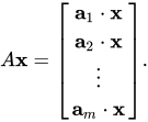
The product Ax can be written in terms of the dot product of vectors as follows: $A\mathbf {x} ={\begin{bmatrix}\mathbf {a} _{1}\cdot \mathbf {x} \\\mathbf {a} _{2}\cdot \mathbf {x} \\\vdots \\\mathbf {a} _{m}\cdot \mathbf {x} \end{bmatrix}}.$

Here, $a 1, ... , a m$ denote the rows of the matrix $A$ . It follows that $x$ is in the kernel of $A$ , if and only if $x$ is orthogonal (or perpendicular) to each of the row vectors of $A$ (since orthogonality is defined as having a dot product of 0).

The row space, or coimage, of a matrix $A$ is the span of the row vectors of $A$ . By the above reasoning, the kernel of $A$ is the orthogonal complement to the row space. That is, a vector $x$ lies in the kernel of $A$ , if and only if it is perpendicular to every vector in the row space of $A$ .

The dimension of the row space of $A$ is called the rank of A, and the dimension of the kernel of $A$ is called the nullity of $A$ . These quantities are related by the rank–nullity theorem^[4] $\operatorname {rank} (A)+\operatorname {nulity} (A)=n.$

Left null space

The left null space, or cokernel, of a matrix $A$ consists of all column vectors $x$ such that $x T A = 0 T$ , where T denotes the transpose of a matrix. The left null space of $A$ is the same as the kernel of $A T$ . The left null space of $A$ is the orthogonal complement to the column space of $A$ , and is dual to the cokernel of the associated linear transformation. The kernel, the row space, the column space, and the left null space of $A$ are the four fundamental subspaces associated with the matrix $A$ .

Nonhomogeneous systems of linear equations

The kernel also plays a role in the solution to a nonhomogeneous system of linear equations: $A\mathbf {x} =\mathbf {b} \quad {\text{or}}\quad {\begin{alignedat}{7}a_{11}x_{1}&&\;+\;&&a_{12}x_{2}&&\;+\;\cdots \;+\;&&a_{1n}x_{n}&&\;=\;&&&b_{1}\\a_{21}x_{1}&&\;+\;&&a_{22}x_{2}&&\;+\;\cdots \;+\;&&a_{2n}x_{n}&&\;=\;&&&b_{2}\\&&&&&&&&&&\vdots \ \;&&&\\a_{m1}x_{1}&&\;+\;&&a_{m2}x_{2}&&\;+\;\cdots \;+\;&&a_{mn}x_{n}&&\;=\;&&&b_{m}\\\end{alignedat}}$ If $u$ and $v$ are two possible solutions to the above equation, then $A(\mathbf {u} -\mathbf {v} )=A\mathbf {u} -A\mathbf {v} =\mathbf {b} -\mathbf {b} =\mathbf {0}$ Thus, the difference of any two solutions to the equation $A x = b$ lies in the kernel of $A$ .

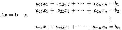
It follows that any solution to the equation $A x = b$ can be expressed as the sum of a fixed solution $v$ and an arbitrary element of the kernel. That is, the solution set to the equation $A x = b$ is $\left\{\mathbf {v} +\mathbf {x} \mid A\mathbf {v} =\mathbf {b} \land \mathbf {x} \in \operatorname {Null} (A)\right\},$ Geometrically, this says that the solution set to $A x = b$ is the translation of the kernel of $A$ by the vector $v$ . See also Fredholm alternative and flat (geometry).

Illustration

The following is a simple illustration of the computation of the kernel of a matrix (see § Computation by Gaussian elimination, below for methods better suited to more complex calculations). The illustration also touches on the row space and its relation to the kernel.

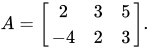
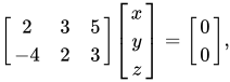
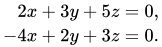
Consider the matrix $A={\begin{bmatrix}2&3&5\\-4&2&3\end{bmatrix}}.$ The kernel of this matrix consists of all vectors $(x, y, z) \in R 3$ for which ${\begin{bmatrix}2&3&5\\-4&2&3\end{bmatrix}}{\begin{bmatrix}x\\y\\z\end{bmatrix}}={\begin{bmatrix}0\\0\end{bmatrix}},$ which can be expressed as a homogeneous system of linear equations involving $x$ , $y$ , and $z$ : ${\begin{aligned}2x+3y+5z&=0,\\-4x+2y+3z&=0.\end{aligned}}$

The same linear equations can also be written in matrix form as: $\left[{\begin{array}{ccc|c}2&3&5&0\\-4&2&3&0\end{array}}\right].$

Through Gauss–Jordan elimination, the matrix can be reduced to: $\left[{\begin{array}{ccc|c}1&0&1/16&0\\0&1&13/8&0\end{array}}\right].$

Rewriting the matrix in equation form yields: ${\begin{aligned}x&=-{\frac {1}{16}}z\\y&=-{\frac {13}{8}}z.\end{aligned}}$

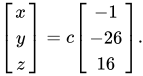
The elements of the kernel can be further expressed in parametric vector form, as follows: ${\begin{bmatrix}x\\y\\z\end{bmatrix}}=c{\begin{bmatrix}-1/16\\-13/8\\1\end{bmatrix}}\quad ({\text{where }}c\in \mathbb {R} )$

Since $c$ is a free variable ranging over all real numbers, this can be expressed equally well as: ${\begin{bmatrix}x\\y\\z\end{bmatrix}}=c{\begin{bmatrix}-1\\-26\\16\end{bmatrix}}.$ The kernel of $A$ is precisely the solution set to these equations (in this case, a line through the origin in $R 3$ ). Here, the vector $(-1,-26,16) T$ constitutes a basis of the kernel of $A$ . The nullity of $A$ is therefore 1, as it is spanned by a single vector.

The following dot products are zero: ${\begin{bmatrix}2&3&5\end{bmatrix}}{\begin{bmatrix}-1\\-26\\16\end{bmatrix}}=0\quad \mathrm {and} \quad {\begin{bmatrix}-4&2&3\end{bmatrix}}{\begin{bmatrix}-1\\-26\\16\end{bmatrix}}=0,$ which illustrates that vectors in the kernel of $A$ are orthogonal to each of the row vectors of $A$ .

These two (linearly independent) row vectors span the row space of $A$ —a plane orthogonal to the vector $(-1,-26,16) T$ .

With the rank 2 of $A$ , the nullity 1 of $A$ , and the dimension 3 of $A$ , we have an illustration of the rank-nullity theorem.

Examples

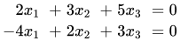
If $L : R m \to R n$ , then the kernel of $L$ is the solution set to a homogeneous system of linear equations. As in the above illustration, if $L$ is the operator: $L(x_{1},x_{2},x_{3})=(2x_{1}+3x_{2}+5x_{3},\;-4x_{1}+2x_{2}+3x_{3})$ then the kernel of $L$ is the set of solutions to the equations ${\begin{alignedat}{7}2x_{1}&\;+\;&3x_{2}&\;+\;&5x_{3}&\;=\;&0\\-4x_{1}&\;+\;&2x_{2}&\;+\;&3x_{3}&\;=\;&0\end{alignedat}}$
Let $C [0,1]$ denote the vector space of all continuous real-valued functions on the interval [0,1], and define $L : C [0,1] \to R$ by the rule $L(f)=f(0.3).$ Then the kernel of $L$ consists of all functions $f \in C [0,1]$ for which $f (0.3) = 0$ .
Let $C \infty (R)$ be the vector space of all infinitely differentiable functions $R \to R$ , and let $D : C \infty (R) \to C \infty (R)$ be the differentiation operator: $D(f)={\frac {df}{dx}}.$ Then the kernel of $D$ consists of all functions in $C \infty (R)$ whose derivatives are zero, i.e. the set of all constant functions.
Let $R \infty$ be the direct product of infinitely many copies of $R$ , and let $s : R \infty \to R \infty$ be the shift operator $s(x_{1},x_{2},x_{3},x_{4},\ldots )=(x_{2},x_{3},x_{4},\ldots ).$ Then the kernel of $s$ is the one-dimensional subspace consisting of all vectors $(x 1, 0, 0, 0, ...)$ .
If $V$ is an inner product space and $W$ is a subspace, the kernel of the orthogonal projection $V \to W$ is the orthogonal complement to $W$ in $V$ .

Computation by Gaussian elimination

La base del núcleo de una matriz se puede calcular mediante la eliminación gaussiana .

Para ello, dada una matriz $A$ $de m \times n$ , primero construimos la matriz aumentada por filas. ${\begin{bmatrix}A\\\hline I\end{bmatrix}},$ donde $I$ es la matriz identidad $n \times n$ .

Calculando su forma escalonada de columna mediante eliminación gaussiana (o cualquier otro método adecuado), obtenemos una matriz ${\begin{bmatrix}B\\\hline C\end{bmatrix}}.$ Una base del núcleo de $A$ consiste en las columnas no nulas de $C$ tales que la columna correspondiente de $B$ es una columna nula .

De hecho, el cálculo puede detenerse tan pronto como la matriz superior esté en forma escalonada por columnas: el resto del cálculo consiste en cambiar la base del espacio vectorial generado por las columnas cuya parte superior es cero.

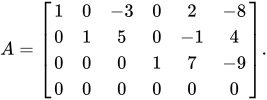
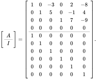
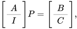
Por ejemplo, supongamos que $A={\begin{bmatrix}1&0&-3&0&2&-8\\0&1&5&0&-1&4\\0&0&0&1&7&-9\\0&0&0&0&0&0\end{bmatrix}}.$ Entonces ${\begin{bmatrix}A\\\hline I\end{bmatrix}}={\begin{bmatrix}1&0&-3&0&2&-8\\0&1&5&0&-1&4\\0&0&0&1&7&-9\\0&0&0&0&0&0\\\hline 1&0&0&0&0&0\\0&1&0&0&0&0\\0&0&1&0&0&0\\0&0&0&1&0&0\\0&0&0&0&1&0\\0&0&0&0&0&1\end{bmatrix}}.$

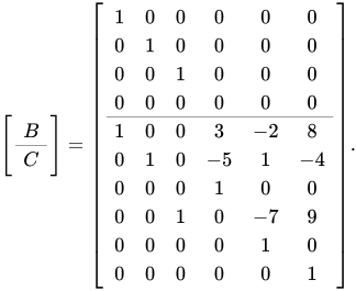
Al colocar la parte superior en forma escalonada de columnas mediante operaciones de columna en toda la matriz se obtiene ${\begin{bmatrix}B\\\hline C\end{bmatrix}}={\begin{bmatrix}1&0&0&0&0&0\\0&1&0&0&0&0\\0&0&1&0&0&0\\0&0&0&0&0&0\\\hline 1&0&0&3&-2&8\\0&1&0&-5&1&-4\\0&0&0&1&0&0\\0&0&1&0&-7&9\\0&0&0&0&1&0\\0&0&0&0&0&1\end{bmatrix}}.$

Las últimas tres columnas de $B$ son columnas cero. Por lo tanto, los tres últimos vectores de $C$ , $\left[\!\!{\begin{array}{r}3\\-5\\1\\0\\0\\0\end{array}}\right],\;\left[\!\!{\begin{array}{r}-2\\1\\0\\-7\\1\\0\end{array}}\right],\;\left[\!\!{\begin{array}{r}8\\-4\\0\\9\\0\\1\end{array}}\right]$ son una base del núcleo de $A.$

Prueba de que el método calcula el núcleo: Dado que las operaciones de columna corresponden a la postmultiplicación por matrices invertibles, el hecho de que ${\begin{bmatrix}A\\\hline I\end{bmatrix}}$ se reduce a ${\begin{bmatrix}B\\\hline C\end{bmatrix}}$ significa que existe una matriz invertible $P$ de tal manera que ${\begin{bmatrix}A\\\hline I\end{bmatrix}}P={\begin{bmatrix}B\\\hline C\end{bmatrix}},$ con $B$ en forma escalonada de columna. Por lo tanto $AP=B$ , $IP=C$ , y $AC=B$ . Un vector columna $\mathbf {v}$ pertenece al núcleo de $A$ (eso es $A\mathbf {v} =\mathbf {0}$ ) si y solo si $B\mathbf {w} =\mathbf {0} ,$ dónde $\mathbf {w} =P^{-1}\mathbf {v} =C^{-1}\mathbf {v}$ . Como $B$ está en forma escalonada de columna, $B\mathbf {w} =\mathbf {0}$ , si y solo si las entradas no nulas de $\mathbf {w}$ corresponden a las columnas cero de $B$ . Multiplicando por $C$ , se puede deducir que este es el caso si y solo si $\mathbf {v} =C\mathbf {w}$ es una combinación lineal de las columnas correspondientes de $C$ .

Cálculo numérico

El problema de calcular el núcleo en un ordenador depende de la naturaleza de los coeficientes.

Coeficientes exactos

Si los coeficientes de la matriz son números exactos, la forma escalonada por columnas de la matriz se puede calcular con el algoritmo de Bareiss de forma más eficiente que con la eliminación gaussiana. Resulta aún más eficiente utilizar la aritmética modular y el teorema chino del resto , lo que reduce el problema a varios problemas similares sobre campos finitos (esto evita la sobrecarga derivada de la no linealidad de la complejidad computacional de la multiplicación de enteros).

Para coeficientes en un campo finito, la eliminación gaussiana funciona bien, pero para las matrices grandes que aparecen en criptografía y en el cálculo de bases de Gröbner , se conocen mejores algoritmos, que tienen aproximadamente la misma complejidad computacional , pero son más rápidos y se comportan mejor con el hardware informático moderno .

Cálculo de punto flotante

Para matrices cuyas entradas son números de punto flotante , el problema de calcular el núcleo solo tiene sentido para matrices cuyo número de filas es igual a su rango: debido a los errores de redondeo , una matriz de punto flotante casi siempre tiene un rango completo , incluso cuando es una aproximación de una matriz de rango mucho menor. Incluso para una matriz de rango completo, es posible calcular su núcleo solo si está bien condicionada , es decir, si tiene un número de condición bajo . ^{[ 5 ]}

Incluso para una matriz de rango completo bien condicionada, la eliminación gaussiana no se comporta correctamente: introduce errores de redondeo demasiado grandes para obtener un resultado significativo. Dado que el cálculo del núcleo de una matriz es un caso particular de resolución de un sistema homogéneo de ecuaciones lineales, el núcleo puede calcularse con cualquiera de los diversos algoritmos diseñados para resolver sistemas homogéneos. Un software de vanguardia para este propósito es la biblioteca Lapack .

Véase también

Notas y referencias

↑ Weisstein, Eric W. "Núcleo" . mathworld.wolfram.com . Consultado el 9 de diciembre de 2019 .
1 2 "Núcleo (espacio nulo) | Brilliant Math & Science Wiki" . brilliant.org . Consultado el 09/12/2019 .
↑ El álgebra lineal, tal como se analiza en este artículo, es una disciplina matemática muy consolidada con numerosas fuentes. Casi todo el material de este artículo se puede encontrar en Lay (2005) , Meyer (2001) y las conferencias de Strang.
1 2 Weisstein, Eric W. "Teorema de rango-nulidad" . mathworld.wolfram.com . Consultado el 9 de diciembre de 2019 .
↑ "Copia archivada" (PDF) . Archivado del original (PDF) el 29-08-2017 . Recuperado el 14-04-2015 .{{cite web}}: CS1 mantenimiento: copia archivada como título ( enlace )

Bibliografía

Axler, Sheldon Jay (1997), Álgebra lineal bien hecha (2.ª ed.), Springer-Verlag, ISBN 0-387-98259-0.
Lay, David C. (2005), Álgebra lineal y sus aplicaciones (3.ª ed.), Addison Wesley, ISBN 978-0-321-28713-7.
Meyer, Carl D. (2001), Análisis matricial y álgebra lineal aplicada , Sociedad de Matemáticas Industriales y Aplicadas (SIAM), ISBN 978-0-89871-454-8Archivado del original el 31 de octubre de 2009.
Poole, David (2006), Álgebra lineal: una introducción moderna (2.ª ed.), Brooks/Cole, ISBN 0-534-99845-3.
Anton, Howard (2005), Álgebra lineal elemental (versión de aplicaciones) (9.ª ed.), Wiley International.
Leon, Steven J. (2006), Álgebra lineal con aplicaciones (7.ª ed.), Pearson Prentice Hall.
Lang, Serge (1987). Álgebra lineal . Springer. ISBN 9780387964126.
Trefethen, Lloyd N.; Bau, David III (1997), Álgebra lineal numérica , SIAM, ISBN 978-0-89871-361-9.

Enlaces externos

"Núcleo de una matriz" , Enciclopedia de Matemáticas , EMS Press , 2001 [1994]
Khan Academy , Introducción al espacio nulo de una matriz

[1] Weisstein, Eric W. "Núcleo" . mathworld.wolfram.com . Consultado el 9 de diciembre de 2019 .

[:0-2] 1 2 "Núcleo (espacio nulo) | Brilliant Math & Science Wiki" . brilliant.org . Consultado el 09/12/2019 .

[textbooks-3] El álgebra lineal, tal como se analiza en este artículo, es una disciplina matemática muy consolidada con numerosas fuentes. Casi todo el material de este artículo se puede encontrar en Lay (2005) , Meyer (2001) y las conferencias de Strang.

[:1-4] 1 2 Weisstein, Eric W. "Teorema de rango-nulidad" . mathworld.wolfram.com . Consultado el 9 de diciembre de 2019 .

[5] "Copia archivada" (PDF) . Archivado del original (PDF) el 29-08-2017 . Recuperado el 14-04-2015 .{{cite web}}: CS1 mantenimiento: copia archivada como título ( enlace )

[

[ 3 ]

[ 5 ]