Articulo de referencia

Quantum phase estimation algorithm

In quantum computing , the quantum phase estimation algorithm is a quantum algorithm to estimate the phase corresponding to an eigenvalue of a given unitary operator . Because t...

In quantum computing, the quantum phase estimation algorithm is a quantum algorithm to estimate the phase corresponding to an eigenvalue of a given unitary operator. Because the eigenvalues of a unitary operator always have unit modulus, they are characterized by their phase, and therefore the algorithm can be equivalently described as retrieving either the phase or the eigenvalue itself. The algorithm was initially introduced by Alexei Kitaev in 1995.[1][2]:246

Phase estimation is frequently used as a subroutine in other quantum algorithms, such as Shor's algorithm,[2]:131 the quantum algorithm for linear systems of equations, and the quantum counting algorithm.

Overview of the algorithm

The algorithm operates on two sets of qubits, referred to in this context as registers. The two registers contain n{\displaystyle n} and m{\displaystyle m} qubits, respectively. Let U{\displaystyle U} be a unitary operator acting on the m{\displaystyle m}-qubit register. The eigenvalues of a unitary operator have unit modulus, and are therefore characterized by their phase. Thus if |ψ{\displaystyle |\psi \rangle } is an eigenvector of U{\displaystyle U}, then U|ψ=e2πiθ|ψ{\displaystyle U|\psi \rangle =e^{2\pi i\theta }\left|\psi \right\rangle } for some θR{\displaystyle \theta \in \mathbb {R} }. Due to the periodicity of the complex exponential, we can always assume 0θ<1{\displaystyle 0\leq \theta <1}.

The goal is producing a good approximation for θ{\displaystyle \theta } with a small number of gates and a high probability of success. The quantum phase estimation algorithm achieves this assuming oracular access to U{\displaystyle U}, and having |ψ{\displaystyle |\psi \rangle } available as a quantum state. This means that when discussing the efficiency of the algorithm we only worry about the number of times U{\displaystyle U} needs to be used, but not about the cost of implementing U{\displaystyle U} itself.

More precisely, the algorithm returns with high probability an approximation for θ{\displaystyle \theta }, within additive error ε{\displaystyle \varepsilon }, using n=O(log(1/ε)){\displaystyle n=O(\log(1/\varepsilon ))} qubits in the first register, and O(1/ε){\displaystyle O(1/\varepsilon)}controlled-U operations. Furthermore, we can improve the success probability to 1Δ{\displaystyle 1-\Delta } for any Δ>0{\displaystyle \Delta >0} by using a total of O(log(1/Δ)/ε){\displaystyle O(\log(1/\Delta )/\varepsilon )} uses of controlled-U, and this is optimal.[3]

Detailed description of the algorithm

The circuit for quantum phase estimation.

State preparation

The initial state of the system is:

|Ψ0=|0n|ψ,{\displaystyle |\Psi _ {0}\rangle =|0\rangle ^{\otimes n}|\psi \rangle ,}

where |ψ{\displaystyle |\psi \rangle } is the m{\displaystyle m}-qubit state that evolves through U{\displaystyle U}. We first apply the n-qubit Hadamard gate operationHn{\displaystyle H^{\otimes n}} on the first register, which produces the state:|Ψ1=(HnIm)|Ψ0=12n2(|0+|1)n|ψ=12n/2j=02n1|j|ψ.{\displaystyle |\Psi _{1}\rangle =(H^{\otimes n}\otimes I_{m})|\Psi _{0}\rangle ={\frac {1}{2^{\frac {n}{2}}}}(|0\rangle +|1\rangle )^{\otimes n}|\psi \rangle ={\frac {1}{2^{n/2}}}\sum _{j=0}^{2^{n}-1}|j\rangle |\psi \rangle .}Note that here we are switching between binary and n{\displaystyle n}representación -aria para lanorte{\displaystyle n}-registro de cúbits: el ket|j{\displaystyle |j\rangle }en el lado derecho es una abreviatura denorte{\displaystyle n}-estado del cúbit|j=0norte1|j{\displaystyle |j\rangle \equiv \bigotimes _{\ell =0}^{n-1}|j_{\ell }\rangle }, dóndej==0norte1j2{\displaystyle j=\sum _{\ell =0}^{n-1}j_{\ell }2^{\ell }}es la descomposición binaria dej{\displaystyle j}.

Operaciones controladas en U

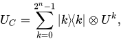
Este estado|Ψ1{\displaystyle |\Psi _ {1}\rangle }Luego evoluciona a través de la evolución unitaria controlada.Udo{\displaystyle U_{C}}cuya acción puede escribirse comoUdo(|k|ψ)=|k(Uk|ψ),{\displaystyle U_{C}(|k\rangle \otimes |\psi \rangle )=|k\rangle \otimes (U^{k}|\psi \rangle ),}a pesar dek=0,...,2norte1{\displaystyle k=0,...,2^{n}-1}Esta evolución también puede escribirse de forma concisa comoUdo=k=02norte1|kk|Uk,{\displaystyle U_{C}=\sum _ {k=0}^{2^{n}-1}|k\rangle \!\langle k|\otimes U^{k},}lo que resalta su naturaleza controlada: se aplicaUk{\displaystyle U^{k}}al segundo registro condicionalmente al primer registro siendo|k{\displaystyle |k\rangle }. Recordando que la condición de autovalor se cumple para|ψ{\displaystyle |\psi \rangle }, aplicandoUdo{\displaystyle U_{C}}a|Ψ1{\displaystyle |\Psi _ {1}\rangle }así da|Ψ2Udo|Ψ1=(12norte/2k=02norte1mi2πiθk|k)|ψ,{\displaystyle |\Psi _{2}\rangle \equiv U_{C}|\Psi _{1}\rangle =\left({\frac {1}{2^{n/2}}}\sum _{k=0}^{2^{n}-1}e^{2\pi i\theta k}|k\rangle \right)\otimes |\psi \rangle ,}donde usamosUk|ψ=mi2πikθ|ψ{\displaystyle U^{k}|\psi \rangle =e^{2\pi ik\theta }|\psi \rangle }.

Para demostrar queUdo{\displaystyle U_{C}}También se puede implementar de manera eficiente, observe que podemos escribirUdo==0norte1do(U2){\displaystyle U_{C}=\prod _{\ell =0}^{n-1}C_{\ell }(U^{2^{\ell }})}, dóndedo(U2){\displaystyle C_{\ell }(U^{2^{\ell }})}denota la operación de aplicaciónU2{\displaystyle U^{2^{\ell }}}al segundo registro condicionalmente al{\displaystyle \ell }-ésimo cúbit del primer registro siendo|1{\displaystyle |1\rangle }Formalmente, estas puertas pueden caracterizarse por su acción comodo(Uk)(|j|ψ)=|j(Ujk|ψ).{\displaystyle C_{\ell }(U^{k})(|j\rangle \otimes |\psi \rangle )=|j\rangle \otimes (U^{j_{\ell }k}|\psi \rangle ).}Esta ecuación puede interpretarse como que el estado permanece sin cambios cuandoj=0{\displaystyle j_{\ell }=0}, es decir, cuando el{\displaystyle \ell }-ésimo cúbit es|0{\displaystyle |0\rangle }, mientras que la puertaUk{\displaystyle U^{k}}se aplica al segundo registro cuando el{\displaystyle \ell }-ésimo cúbit es|1{\displaystyle |1\rangle }La composición de estas compuertas controladas da como resultado=0norte1do(U2)(|j|ψ)=|j(U=0norte1j2|ψ)=Udo(|j|ψ),{\displaystyle \prod _{\ell =0}^{n-1}C_{\ell }(U^{2^{\ell }})(|j\rangle \otimes |\psi \rangle )=|j\rangle \otimes \left(U^{\sum _{\ell =0}^{n-1}j_{\ell }2^{\ell }}|\psi \rangle \right)=U_{C}\left(|j\rangle \otimes |\psi \rangle \right),}con el último paso directamente derivado de la descomposición binariaj==0norte1j2{\displaystyle j=\sum _{\ell =0}^{n-1}j_{\ell }2^{\ell }}.

A partir de este punto, el segundo registro queda intacto, y por lo tanto es conveniente escribir|Ψ2=|Ψ~2|ψ{\displaystyle |\Psi _{2}\rangle =|{\tilde {\Psi }}_{2}\rangle \otimes |\psi \rangle }, con|Ψ~2{\displaystyle |{\tilde {\Psi }}_{2}\rangle }el estado de lanorte{\displaystyle n}-registro de cúbits, que es el único que necesitamos considerar para el resto del algoritmo.

Aplicar la transformada cuántica inversa de Fourier

La parte final del circuito implica la aplicación de la transformada cuántica inversa de Fourier (QFT).QFT{\displaystyle {\mathcal {QFT}}}en el primer registro de|Ψ2{\displaystyle |\Psi _{2}\rangle }:|Ψ~3=QFT2norte1|Ψ~2.{\displaystyle |{\tilde {\Psi }}_{3}\rangle ={\mathcal {QFT}}_{2^{n}}^{-1}|{\tilde {\Psi }}_{2}\rangle .}La QFT y su inversa se caracterizan por su acción sobre los estados base comoQFTnorte|k=norte1/2j=0norte1mi2πinortejk|j,QFTnorte1|k=norte1/2j=0norte1mi2πinortejk|j.{\displaystyle {\begin{aligned}{\mathcal {QFT}}_{N}|k\rangle &=N^{-1/2}\sum _{j=0}^{N-1}e^{{\frac {2\pi i}{N}}jk}|j\rangle ,\\{\mathcal {QFT}}_{N}^{-1}|k\rangle &=N^{-1/2}\sum _{j=0}^{N-1}e^{-{\frac {2\pi i}{N}}jk}|j\rangle .\end{aligned}}}Resulta que

|Ψ~3=12norte2k=02norte1mi2πiθk(12norte2incógnita=02norte1mi2πikincógnita2norte|incógnita)=12norteincógnita=02norte1k=02norte1mi2πik2norte(incógnita2norteθ)|incógnita.{\displaystyle |{\tilde {\Psi }}_{3}\rangle ={\frac {1}{2^{\frac {n}{2}}}}\sum _{k=0}^{2^{n}-1}e^{2\pi i\theta k}\left({\frac {1}{2^{\frac {n}{2}}}}\sum _{x=0}^{2^{n}-1}e^{\frac {-2\pi ikx}{2^{n}}}|x\rangle \right)={\frac {1}{2^{n}}}\sum _{x=0}^{2^{n}-1}\sum _{k=0}^{2^{n}-1}e^{-{\frac {2\pi ik}{2^{n}}}\left(x-2^{n}\theta \right)}|x\rangle .}

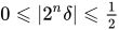
Descomponiendo el estado en la base computacional como|Ψ~3=incógnita=02norte1doincógnita|incógnita,{\textstyle |{\tilde {\Psi }}_{3}\rangle =\sum _{x=0}^{2^{n}-1}c_{x}|x\rangle ,}los coeficientes son, por lo tanto, igualesdoincógnita12nortek=02norte1mi2πik2norte(incógnita2norteθ)=12nortek=02norte1mi2πik2norte(incógnitaa)mi2πiδk,{\displaystyle c_{x}\equiv {\frac {1}{2^{n}}}\sum _{k=0}^{2^{n}-1}e^{-{\frac {2\pi ik}{2^{n}}}(x-2^{n}\theta )}={\frac {1}{2^{n}}}\sum _{k=0}^{2^{n}-1}e^{-{\frac {2\pi ik}{2^{n}}}\left(x-a\right)}e^{2\pi i\delta k},}donde escribimos2norteθ=a+2norteδ,{\displaystyle 2^{n}\theta =a+2^{n}\delta ,}cona{\displaystyle a}es el entero más cercano a2norteθ{\displaystyle 2^{n}\theta }La diferencia2norteδ{\displaystyle 2^{n}\delta } debe por definición satisfacer0|2norteδ|12{\displaystyle 0\leqslant |2^{n}\delta |\leqslant {\tfrac {1}{2}}}Esto equivale a aproximar el valor deθ[0,1]{\displaystyle \theta \in [0,1]}redondeando2norteθ{\displaystyle 2^{n}\theta }al entero más cercano.

Medición

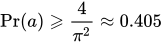
El paso final consiste en realizar una medición en la base computacional en el primer registro. Esto produce el resultado.|y{\displaystyle |y\rangle }con probabilidadPr(y)=|doy|2=|12nortek=02norte1mi2πik2norte(ya)mi2πiδk|2.{\displaystyle \Pr(y)=|c_{y}|^{2}=\left|{\frac {1}{2^{n}}}\sum _{k=0}^{2^{n}-1}e^{{\frac {-2\pi ik}{2^{n}}}(y-a)}e^{2\pi i\delta k}\right|^{2}.}Resulta quePr(a)=1{\displaystyle \operatorname {Pr} (a)=1}siδ=0{\displaystyle \delta =0}, es decir, cuandoθ{\displaystyle \theta }se puede escribir comoθ=a/2norte{\displaystyle \theta =a/2^{n}}Siempre se encuentra el resultadoy=a{\displaystyle y=a}. Por otro lado, siδ0{\displaystyle \delta \neq 0}, la probabilidad dicePr(a)=122norte|k=02norte1mi2πiδk|2=122norte|1mi2πi2norteδ1mi2πiδ|2.{\displaystyle \operatorname {Pr} (a)={\frac {1}{2^{2n}}}\left|\sum _{k=0}^{2^{n}-1}e^{2\pi i\delta k}\right|^{2}={\frac {1}{2^{2n}}}\left|{\frac {1-{e^{2\pi i2^{n}\delta }}}{1-{e^{2\pi i\delta }}}}\right|^{2}.}De esta expresión podemos ver quePr(a)4π20,405{\displaystyle \Pr(a)\geqslant {\frac {4}{\pi ^{2}}}\approx 0.405}cuandoδ0{\displaystyle \delta \neq 0}Para ver esto, observamos que a partir de la definición deδ{\displaystyle \delta }tenemos la desigualdad|δ|12norte+1{\displaystyle |\delta |\leqslant {\tfrac {1}{2^{n+1}}}}y así: [ 4 ] : 157 [ 5 ] : 348Pr(a)=122norte|1mi2πi2norteδ1mi2πiδ|2para δ0=122norte|2pecado(π2norteδ)2pecado(πδ)|2|1mi2iincógnita|2=4|pecado(incógnita)|2=122norte|pecado(π2norteδ)|2|pecado(πδ)|2122norte|pecado(π2norteδ)|2|πδ|2|pecado(πδ)||πδ|122norte|22norteδ|2|πδ|2|22norteδ||pecado(π2norteδ)| para |δ|12norte+14π2.{\displaystyle {\begin{aligned}\Pr(a)&={\frac {1}{2^{2n}}}\left|{\frac {1-{e^{2\pi i2^{n}\delta }}}{1-{e^{2\pi i\delta }}}}\right|^{2}&&{\text{for }}\delta \neq 0\\&={\frac {1}{2^{2n}}}\left|{\frac {2\sin \left(\pi 2^{n}\delta \right)}{2\sin(\pi \delta )}}\right|^{2}&&\left|1-e^{2ix}\right|^{2}=4\left|\sin(x)\right|^{2}\\&={\frac {1}{2^{2n}}}{\frac {\left|\sin \left(\pi 2^{n}\delta \right)\right|^{2}}{|\sin(\pi \delta )|^{2}}}\\&\geqslant {\frac {1}{2^{2n}}}{\frac {\left|\sin \left(\pi 2^{n}\delta \right)\right|^{2}}{|\pi \delta |^{2}}}&&|\sin(\pi \delta )|\leqslant |\pi \delta |\\&\geqslant {\frac {1}{2^{2n}}}{\frac {|2\cdot 2^{n}\delta |^{2}}{|\pi \delta |^{2}}}&&|2\cdot 2^{n}\delta |\leqslant |\sin(\pi 2^{n}\delta )|{\text{ for }}|\delta |\leqslant {\frac {1}{2^{n+1}}}\\&\geqslant {\frac {4}{\pi ^{2}}}.\end{aligned}}}

Concluimos que el algoritmo proporciona el mejornorte{\displaystyle n}estimación de bits (es decir, una que esté dentro1/2norte{\displaystyle 1/2^{n}}de la respuesta correcta) deθ{\displaystyle \theta }con probabilidad al menos4/π2{\displaystyle 4/\pi ^{2}}. Al agregar una cantidad de cúbits adicionales del orden deO(registro(1/ϵ)){\displaystyle O(\log(1/\epsilon ))}y truncando los cúbits adicionales la probabilidad puede aumentar a1ϵ{\displaystyle 1-\epsilon }. [ 5 ]

Ejemplos de juguetes

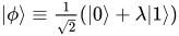
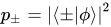
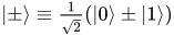
Consideremos la instancia más simple posible del algoritmo, donde solonorte=1{\displaystyle n=1}cúbito, además de los cúbitos necesarios para codificar|ψ{\displaystyle |\psi \rangle }, está involucrado. Supongamos que el valor propio de|ψ{\displaystyle |\psi \rangle }lecturasλ=mi2πiθ{\displaystyle \lambda =e^{2\pi i\theta }},θ[0,1){\displaystyle \theta \in [0,1)}La primera parte del algoritmo genera el estado de un cúbit.|ϕ12(|0+λ|1){\textstyle |\phi \rangle \equiv {\frac {1}{\sqrt {2}}}(|0\rangle +\lambda |1\rangle )}. Aplicando la QFT inversa se obtienen en este caso aplicando una puerta de Hadamard . Las probabilidades del resultado final son, por lo tanto,pag±=|±|ϕ|2{\displaystyle p_{\pm }=|\langle \pm |\phi \rangle |^{2}}dónde|±12(|0±|1){\textstyle |\pm \rangle \equiv {\frac {1}{\sqrt {2}}}(|0\rangle \pm |1\rangle )}, o más explícitamente,pag±=|1±λ|24=1±porque(2πθ)2.{\displaystyle p_{\pm }={\frac {|1\pm \lambda |^{2}}{4}}={\frac {1\pm \cos(2\pi \theta )}{2}}.}Suponerλ=1{\displaystyle \lambda =1}, significado|ϕ=|+{\displaystyle |\phi \rangle =|+\rangle }. Entoncespag+=1{\displaystyle p_{+}=1},pag=0{\displaystyle p_{-}=0}y recuperamos de forma determinista el valor preciso deλ{\displaystyle \lambda }a partir de los resultados de la medición. Lo mismo se aplica siλ=1{\displaystyle \lambda =-1}.

Si por otro ladoλ=mi2πi/3{\displaystyle \lambda =e^{2\pi i/3}}, entoncespag±=[1±porque(2π/3)]/2{\displaystyle p_{\pm }=[1\pm \cos(2\pi /3)]/2}, eso es,pag+=1/4{\displaystyle p_{+}=1/4}ypag=3/4{\displaystyle p_{-}=3/4}En este caso, el resultado no es determinista, pero aun así encontramos el resultado.|{\displaystyle |-\rangle }como más probable, compatible con el hecho de que2/3{\displaystyle 2/3}está más cerca de 1 que de 0.

En términos más generales, siλ=mi2πiθ{\displaystyle \lambda =e^{2\pi i\theta }}, entoncespag+1/2{\displaystyle p_{+}\geq 1/2}si y solo si|θ|1/4{\displaystyle |\theta |\leq 1/4}Esto es consistente con los resultados anteriores porque en los casosλ=±1{\displaystyle \lambda =\pm 1}, correspondiente aθ=0,1/2{\displaystyle \theta =0,1/2}La fase se recupera de forma determinista, y las demás fases se recuperan con mayor precisión cuanto más cerca estén de estas dos.

Véase también

Referencias

  1. Kitaev, A. Yu (1995-11-20). "Mediciones cuánticas y el problema del estabilizador abeliano". arXiv : quant-ph/9511026 .
  2. 1 2 Nielsen, Michael A. y Isaac L. Chuang (2001). Computación cuántica e información cuántica (Ed. reimpresa ). Cambridge [ua]: Cambridge Univ. Press. ISBN  978-0521635035.
  3. Mande, Nikhil S.; Ronald de Wolf (2023). "Límites ajustados para la estimación de fase cuántica y problemas relacionados". arXiv : 2305.04908 [ quant-ph ].
  4. ^ Benenti, Giuliano; Casati, Giulio; Strini, Giuliano (2004). Principios de información y computación cuántica (Reimpreso. Ed.). Nueva Jersey [ua]: Científico mundial. ISBN  978-9812388582.
  5. 1 2 Cleve, R.; Ekert, A.; Macchiavello, C.; Mosca, M. (8 de enero de 1998). "Algoritmos cuánticos revisados". Actas de la Royal Society A: Ciencias Matemáticas, Físicas y de Ingeniería . 454 (1969): 339– 354. arXiv : quant-ph/9708016 . Bibcode : 1998RSPSA.454..339C . doi : 10.1098/rspa.1998.0164 . S2CID 16128238 .