 Hispanopedia Wiki
In electrical circuit theory, the zero state response (ZSR) is the behaviour or response of a circuit with initial state of zero. The ZSR results only from the external inputs or driving functions of the circuit and not from the initial state.[1]
The total response of the circuit is the superposition of the ZSR and the ZIR, or Zero Input Response. The ZIR results only from the initial state of the circuit and not from any external drive. The ZIR is also called the natural response, and the resonant frequencies of the ZIR are called the natural frequencies. Given a description of a system in the s-domain, the zero-state response can be described as Y(s)=Init(s)/a(s) where a(s) and Init(s) are system-specific.
Zero state response and zero input response in integrator and differentiator circuits
One example of zero state response being used is in integrator and differentiator circuits. By examining a simple integrator circuit it can be demonstrated that when a function is put into a linear time-invariant (LTI) system, an output can be characterized by a superposition or sum of the Zero Input Response and the zero state response.
A system can be represented as


with the input on the left and the output on the right.


The output can be separated into a zero input and a zero state solution with
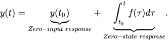
The contributions of and to output are additive and each contribution and vanishes with vanishing and


This behavior constitutes a linear system. A linear system has an output that is a sum of distinct zero-input and zero-state components, each varying linearly, with the initial state of the system and the input of the system respectively.
The zero input response and zero state response are independent of each other and therefore each component can be computed independently of the other.
Zero state response in integrator and differentiator circuits
The Zero State Response represents the system output when

When there is no influence from internal voltages or currents due to previously charged components
Zero state response varies with the system input and under zero-state conditions we could say that two independent inputs results in two independent outputs:


and


Because of linearity we can then apply the principles of superposition to achieve


Verifications of zero state response in integrator and differentiator circuits
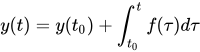
To arrive at general equation

The circuit to the right acts as a simple integrator circuit and will be used to verify the equation as the zero state response of an integrator circuit.
Los condensadores tienen la relación corriente-voltaje donde C es la capacitancia, medida en faradios , del condensador.

Manipulando la ecuación anterior, se puede demostrar que el condensador integra eficazmente la corriente que lo atraviesa. La ecuación resultante también muestra las respuestas de estado cero y de entrada cero del circuito integrador.
Primero, integrando ambos lados de la ecuación anterior
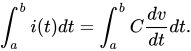
Segundo, integrando el lado derecho
![{\displaystyle \int _{a}^{b}i(t)dt=C[v(b)-v(a)].}](https://wikimedia.org/api/rest_v1/media/math/render/svg/0429c41f70fb7aab08c1c14d5d001c4ce6796794)
En tercer lugar, distribuye y resta.Llegar

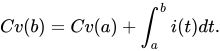
Cuarto, divide porlograr

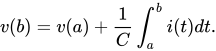
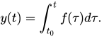
Al sustituirparayparay mediante el uso de la variable ficticiacomo variable de integración la ecuación general


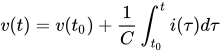
se encuentra.
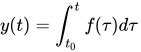
Para llegar a un ejemplo específico del circuito
La ecuación general puede utilizarse entonces para demostrar aún más esta verificación utilizando las condiciones del circuito integrador simple descrito anteriormente.
Utilizando una capacitancia de 1 faradio como se muestra en el circuito integrador anterior
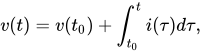
que es la ecuación que contiene la entrada cero y la respuesta de estado cero que se ve en la parte superior de la página.
Para verificar la linealidad del estado cero
Para verificar su linealidad en estado cero, establezca el voltaje alrededor del condensador en el tiempo 0 igual a 0, o, lo que significa que no hay voltaje inicial. Esto elimina el primer término que forma la ecuación.

.
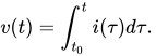
De acuerdo con los métodos de sistemas lineales invariantes en el tiempo , al introducir dos entradas diferentes en el circuito integrador,y, las dos salidas diferentes


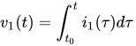
y
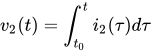
se encuentran respectivamente.
Mediante el uso del principio de superposición, las entradasyse pueden combinar para obtener una nueva entrada

y una nueva salida

Al integrar el lado derecho de


se encuentra, lo que implica que el sistema es lineal en el estado cero,.
Este ejemplo de verificación también podría haberse realizado con una fuente de voltaje en lugar de la fuente de corriente y un inductor en lugar del condensador. En ese caso, habríamos estado calculando una corriente en lugar de un voltaje.
La industria de respuesta de estado cero utiliza
El método de análisis de circuitos, que consiste en descomponer la salida de un sistema en un estado cero y una respuesta de entrada cero, se utiliza ampliamente en la industria, incluyendo circuitos , sistemas de control , procesamiento de señales y electromagnetismo . Además, la mayoría del software de simulación de circuitos , como SPICE , admite este método de una u otra forma.
Referencias
- ↑ "Entrada cero y respuesta de estado cero" . lpsa.swarthmore.edu . Consultado el 10 de noviembre de 2025 .
Enlaces externos
- Electrotecnia


