 Hispanopedia Wiki
En teoría de la probabilidad y estadística , la distribución beta es una familia de distribuciones de probabilidad continuas definidas en el intervalo [0, 1] o (0, 1) en términos de dos parámetros positivos , denotados por alfa ( α ) y beta ( β ), que aparecen como exponentes de la variable y su complemento a 1, respectivamente, y controlan la forma de la distribución.
La distribución beta se ha aplicado para modelar el comportamiento de variables aleatorias limitadas a intervalos de longitud finita en una amplia variedad de disciplinas. La distribución beta es un modelo adecuado para el comportamiento aleatorio de porcentajes y proporciones.
En la inferencia bayesiana , la distribución beta es la distribución de probabilidad a priori conjugada para las distribuciones de Bernoulli , binomial , binomial negativa y geométrica .
La formulación de la distribución beta que se analiza aquí también se conoce como distribución beta de primera especie , mientras que la distribución beta de segunda especie es un nombre alternativo para la distribución beta prima . La generalización a múltiples variables se denomina distribución de Dirichlet .
Definiciones
Función de densidad de probabilidad

La función de densidad de probabilidad (FDP) de la distribución beta, paraoy parámetros de forma,es una función potencial de la variabley de su reflexióncomo sigue:


![{\displaystyle {\begin{aligned}f(x;\alpha ,\beta )&=\mathrm {constant} \cdot x^{\alpha -1}(1-x)^{\beta -1}\\[3pt]&={\frac {x^{\alpha -1}(1-x)^{\beta -1}}{\displaystyle \int _{0}^{1}u^{\alpha -1}(1-u)^{\beta -1}\,du}}\\[6pt]&={\frac {\Gamma (\alpha +\beta )}{\Gamma (\alpha )\Gamma (\beta )}}\,x^{\alpha -1}(1-x)^{\beta -1}\\[6pt]&={\frac {1}{\mathrm {B} (\alpha ,\beta )}}x^{\alpha -1}(1-x)^{\beta -1}\end{aligned}}}](https://wikimedia.org/api/rest_v1/media/math/render/svg/5fc18388353b219c482e8e35ca4aae808ab1be81)
dóndees la función gamma . La función beta ,, es una constante de normalización para asegurar que la probabilidad total sea 1. En las ecuaciones anterioreses una realización —un valor observado que realmente ocurrió— de una variable aleatoria.


Varios autores, entre ellos NL Johnson y S. Kotz , [ 1 ] utilizan los símbolosy(en lugar dey) para los parámetros de forma de la distribución beta, que recuerdan a los símbolos tradicionalmente utilizados para los parámetros de la distribución de Bernoulli , porque la distribución beta se aproxima a la distribución de Bernoulli en el límite cuando ambos parámetros de formayacercarse a cero.


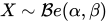
A continuación, una variable aleatoriadistribución beta con parámetrosyse denotará por: [ 2 ] [ 3 ]

Otras notaciones para variables aleatorias con distribución beta utilizadas en la literatura estadística son:[ 4 ] y. [ 5 ]

Función de distribución acumulativa


La función de distribución acumulativa es

dóndees la función beta incompleta yes la función beta incompleta regularizada .


Para enteros positivos α y β , la función de distribución acumulativa de una distribución beta se puede expresar en términos de la función de distribución acumulativa de una distribución binomial con [ 6 ].

Parametrizaciones alternativas
Dos parámetros
Media y tamaño de la muestra
La distribución beta también puede ser reparametrizada en términos de su media μ (0 < μ < 1) y la suma de los dos parámetros de forma ν = α + β > 0 ( [ 3 ] p. 83). Denotando por αPosterior y βPosterior los parámetros de forma de la distribución beta posterior resultante de aplicar el teorema de Bayes a una función de verosimilitud binomial y una probabilidad previa, la interpretación de la suma de ambos parámetros de forma como tamaño de muestra = ν = α ·Posterior + β ·Posterior es solo correcta para la probabilidad previa de Haldane Beta(0,0). Específicamente, para la probabilidad previa bayesiana (uniforme) Beta(1,1) la interpretación correcta sería tamaño de muestra = α ·Posterior + β Posterior − 2, o ν = (tamaño de muestra) + 2. Para tamaños de muestra mucho mayores que 2, la diferencia entre estas dos probabilidades previas se vuelve insignificante. (Consulte la sección Inferencia bayesiana para obtener más detalles). ν = α + β se denomina "tamaño de la muestra" de una distribución beta, pero conviene recordar que, estrictamente hablando, es el "tamaño de la muestra" de una función de verosimilitud binomial solo cuando se utiliza una distribución previa Haldane Beta(0,0) en el teorema de Bayes.
Esta parametrización puede ser útil en la estimación de parámetros bayesianos. Por ejemplo, se puede administrar una prueba a varios individuos. Si se supone que la puntuación de cada persona (0 ≤ θ ≤ 1) se extrae de una distribución beta a nivel poblacional, entonces una estadística importante es la media de esta distribución a nivel poblacional. Los parámetros de media y tamaño de la muestra están relacionados con los parámetros de forma α y β a través de [ 3 ].
Bajo esta parametrización , se puede colocar una probabilidad previa no informativa sobre la media y una probabilidad previa vaga (como una distribución exponencial o gamma ) sobre los números reales positivos para el tamaño de la muestra, si son independientes y los datos y/o creencias previos lo justifican.
Modo y concentración
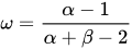
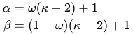
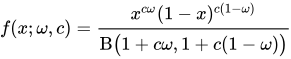
Distribuciones beta cóncavas , que tienen, puede parametrizarse en términos de modo y "concentración". El modo,y concentración,, se puede utilizar para definir los parámetros de forma habituales de la siguiente manera: [ 7 ] Para el modo,Para estar bien definidos, necesitamoso equivalentemente. Si en cambio definimos la concentración como, la condición se simplifica ay la densidad beta enyse puede escribir como: dóndeescala directamente las estadísticas suficientes ,y. Nótese también que en el límite,La distribución se vuelve plana.










Media y varianza
Resolviendo el sistema de ecuaciones (acopladas) dado en las secciones anteriores como las ecuaciones para la media y la varianza de la distribución beta en términos de los parámetros originales α y β , se pueden expresar los parámetros α y β en términos de la media ( μ ) y la varianza (var):
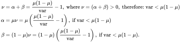
Esta parametrización de la distribución beta puede conducir a una comprensión más intuitiva que la basada en los parámetros originales α y β . Por ejemplo, al expresar la moda, la asimetría, la curtosis excesiva y la entropía diferencial en términos de la media y la varianza:


Cuatro parámetros
Una distribución beta con los dos parámetros de forma α y β tiene soporte en el rango [0,1] o (0,1). Es posible alterar la ubicación y la escala de la distribución introduciendo dos parámetros adicionales que representan los valores mínimo, a , y máximo c ( c > a ), de la distribución, [ 1 ] mediante una transformación lineal que sustituye la variable adimensional x en términos de la nueva variable y (con soporte [ a , c ] o ( a , c )) y los parámetros a y c :

La función de densidad de probabilidad de la distribución beta de cuatro parámetros es igual a la distribución de dos parámetros, escalada por el rango ( c − a ), (de modo que el área total bajo la curva de densidad sea igual a una probabilidad de uno), y con la variable "y" desplazada y escalada de la siguiente manera:
![{\displaystyle {\begin{aligned}f(y;\alpha ,\beta ,a,c)={\frac {f(x;\alpha ,\beta )}{c-a}}&={\frac {\left({\frac {y-a}{c-a}}\right)^{\alpha -1}\left({\frac {c-y}{c-a}}\right)^{\beta -1}}{(c-a)B(\alpha ,\beta )}}\\[1ex]&={\frac {(y-a)^{\alpha -1}(c-y)^{\beta -1}}{(c-a)^{\alpha +\beta -1}B(\alpha ,\beta )}}.\end{aligned}}}](https://wikimedia.org/api/rest_v1/media/math/render/svg/ebfbb9c4da37593762747522d2d91a4ca72e0011)
Que una variable aleatoria Y tenga una distribución beta con cuatro parámetros α , β , a y c se denotará por:

Algunas medidas de ubicación central se escalan (por ( c − a )) y se desplazan (por a ), de la siguiente manera:
![{\displaystyle {\begin{aligned}\mu _{Y}&=\mu _{X}(c-a)+a\\[1ex]&={\frac {\alpha }{\alpha +\beta }}\left(c-a\right)+a={\frac {\alpha c+\beta a}{\alpha +\beta }}\end{aligned}}}](https://wikimedia.org/api/rest_v1/media/math/render/svg/86a8b4fe30b5075b8c038d5b5b3e1f6ee8e5963f)
![{\displaystyle {\begin{aligned}{\text{mode}}(Y)&={\text{mode}}(X)(c-a)+a\\[1ex]&={\frac {\alpha -1}{\alpha +\beta -2}}\left(c-a\right)+a\\[1ex]&={\frac {(\alpha -1)c+(\beta -1)a}{\alpha +\beta -2}}\ ,&{\text{ if }}\alpha ,\,\beta >1\end{aligned}}}](https://wikimedia.org/api/rest_v1/media/math/render/svg/768c42362dbb2d2904c218dcfc6df1de62b5f635)
![{\displaystyle {\begin{aligned}{\text{median}}(Y)&={\text{median}}(X)(c-a)+a\\[1ex]&=I_{\frac {1}{2}}^{[-1]}(\alpha ,\beta )\left(c-a\right)+a\end{aligned}}}](https://wikimedia.org/api/rest_v1/media/math/render/svg/9b039773a1da5743c1e27109447176e3cfe1925e)
Nota: la media geométrica y la media armónica no se pueden transformar mediante una transformación lineal como sí se puede hacer con la media, la mediana y la moda.
Los parámetros de forma de Y se pueden escribir en términos de su media y varianza como

Las medidas de dispersión estadística se escalan (no es necesario desplazarlas porque ya están centradas en la media) por el rango ( c − a ), linealmente para la desviación media y no linealmente para la varianza:
![{\displaystyle {\begin{aligned}&{\text{(mean deviation around mean)}}(Y)\\[1ex]&=({\text{(mean deviation around mean)}}(X))(c-a)\\&={\frac {2\alpha ^{\alpha }\beta ^{\beta }}{\mathrm {B} (\alpha ,\beta )(\alpha +\beta )^{\alpha +\beta +1}}}(c-a)\end{aligned}}}](https://wikimedia.org/api/rest_v1/media/math/render/svg/769fc1182a10805b989db4ae5c207769240dc3b5)

Dado que la asimetría y la curtosis excesiva son cantidades adimensionales (como momentos centrados en la media y normalizados por la desviación estándar ), son independientes de los parámetros a y c , y por lo tanto son iguales a las expresiones dadas anteriormente en términos de X (con soporte [0,1] o (0,1)):

![{\displaystyle {\text{kurtosis excess}}(Y)={\text{kurtosis excess}}(X)={\frac {6\left[(\alpha -\beta )^{2}(\alpha +\beta +1)-\alpha \beta (\alpha +\beta +2)\right]}{\alpha \beta (\alpha +\beta +2)(\alpha +\beta +3)}}}](https://wikimedia.org/api/rest_v1/media/math/render/svg/76f8b524c994e9cdaf8317555457b4369ab2271e)
Propiedades
Medidas de tendencia central
Modo
La moda de una variable aleatoria X con distribución beta con α , β > 1 es el valor más probable de la distribución (correspondiente al pico en la PDF), y viene dada por la siguiente expresión: [ 1 ]

Cuando ambos parámetros son menores que uno ( α , β < 1), este es el antimodo: el punto más bajo de la curva de densidad de probabilidad. [ 8 ]
Si hacemos α = β , la expresión para la moda se simplifica a 1/2, lo que muestra que para α = β > 1 la moda (o antimoda cuando α , β < 1 ) está en el centro de la distribución: es simétrica en esos casos. Consulte la sección Formas en este artículo para obtener una lista completa de los casos de moda, para valores arbitrarios de α y β . Para varios de estos casos, el valor máximo de la función de densidad ocurre en uno o ambos extremos. En algunos casos, el valor (máximo) de la función de densidad que ocurre en el extremo es finito. Por ejemplo, en el caso de α = 2, β = 1 (o α = 1, β = 2), la función de densidad se convierte en una distribución de triángulo rectángulo que es finita en ambos extremos. En varios otros casos hay una singularidad en un extremo, donde el valor de la función de densidad se aproxima al infinito. Por ejemplo, en el caso α = β = 1/2, la distribución beta se simplifica a la distribución arcoseno . Existe un debate entre los matemáticos sobre algunos de estos casos y si los extremos ( x = 0 y x = 1) pueden llamarse modas o no. [ 9 ] [ 2 ]

- Si los extremos forman parte del dominio de la función de densidad
- Si una singularidad puede ser llamada alguna vez un modo
- Si los casos con dos máximos deben denominarse bimodales.
Mediana


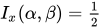
La mediana de la distribución beta es el único número realpara la cual la función beta incompleta regularizadaNo existe una expresión general en forma cerrada para la mediana de la distribución beta para valores arbitrarios de α y β . A continuación se presentan expresiones en forma cerrada para valores particulares de los parámetros α y β :
![{\displaystyle x=I_{1/2}^{[-1]}(\alpha ,\beta )}](https://wikimedia.org/api/rest_v1/media/math/render/svg/d7510f94efa49f254eb3924678b527a6fd22d0fc)
- Para casos simétricos α = β , mediana = 1/2.
- Para α = 1 y β > 0, mediana(Este caso es la imagen especular de la distribución de la función de potencia )
- Para α > 0 y β = 1, mediana =(este caso es la distribución de función de potencia [ 9 ] )
- Para α = 3 y β = 2, mediana = 0,6142724318676105..., la solución real de la ecuación cuártica 1 − 8 x 3 + 6 x 4 = 0, que se encuentra en [0,1].
- Para α = 2 y β = 3, mediana = 0,38572756813238945... = 1−mediana(Beta(3, 2))


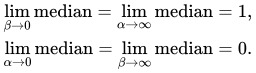
Los siguientes son los límites con un parámetro finito (distinto de cero) y el otro aproximándose a estos límites:
Una aproximación razonable del valor de la mediana de la distribución beta, para α y β mayores o iguales a uno, viene dada por la fórmula [ 10 ].
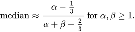
Cuando α , β ≥ 1, el error relativo (el error absoluto dividido por la mediana) en esta aproximación es menor al 4% y para ambos α ≥ 2 y β ≥ 2 es menor al 1%. El error absoluto dividido por la diferencia entre la media y la moda es igualmente pequeño:
![Abs[(Median-Appr.)/Median] for beta distribution for 1 ≤ α ≤ 5 and 1 ≤ β ≤ 5](https://images.hispanopedia.wiki/wikipedia/commons/thumb/a/af/Relative_Error_for_Approximation_to_Median_of_Beta_Distribution_for_alpha_and_beta_from_1_to_5_-_J._Rodal.jpg/500px-Relative_Error_for_Approximation_to_Median_of_Beta_Distribution_for_alpha_and_beta_from_1_to_5_-_J._Rodal.jpg)
![Abs[(Median-Appr.)/(Mean-Mode)] for beta distribution for 1 ≤ α ≤ 5 and 1 ≤ β ≤ 5](https://images.hispanopedia.wiki/wikipedia/commons/thumb/e/e8/Error_in_Median_Apprx._relative_to_Mean-Mode_distance_for_Beta_Distribution_with_alpha_and_beta_from_1_to_5_-_J._Rodal.jpg/500px-Error_in_Median_Apprx._relative_to_Mean-Mode_distance_for_Beta_Distribution_with_alpha_and_beta_from_1_to_5_-_J._Rodal.jpg)
Significar

El valor esperado (media) ( μ ) de una variable aleatoria X con distribución beta y dos parámetros α y β es una función únicamente de la razón β / α de estos parámetros: [ 1 ]
![{\displaystyle {\begin{aligned}\mu =\operatorname {E} [X]&=\int _{0}^{1}xf(x;\alpha ,\beta )\,dx\\&=\int _{0}^{1}x\,{\frac {x^{\alpha -1}(1-x)^{\beta -1}}{\mathrm {B} (\alpha ,\beta )}}\,dx\\&={\frac {\alpha }{\alpha +\beta }}\\&={\frac {1}{1+{\frac {\beta }{\alpha }}}}\end{aligned}}}](https://wikimedia.org/api/rest_v1/media/math/render/svg/e9137834d9d47360ed6c23550c6236fed5fd35f7)
Si hacemos α = β en la expresión anterior, obtenemos μ = 1/2 , lo que demuestra que para α = β la media se encuentra en el centro de la distribución: es simétrica. Además, a partir de la expresión anterior se pueden obtener los siguientes límites:

Por lo tanto, para β / α → 0, o para α / β → ∞, la media se encuentra en el extremo derecho, x = 1. Para estas razones límite, la distribución beta se convierte en una distribución degenerada de un punto con un pico de la función delta de Dirac en el extremo derecho, x = 1 , con probabilidad 1, y probabilidad cero en cualquier otro lugar. Hay una probabilidad del 100% (certeza absoluta) concentrada en el extremo derecho, x = 1 .
De forma similar, para β / α → ∞, o para α / β → 0, la media se sitúa en el extremo izquierdo, x = 0. La distribución beta se convierte en una distribución degenerada de un punto con un pico de función delta de Dirac en el extremo izquierdo, x = 0, con probabilidad 1, y probabilidad cero en cualquier otro lugar. Hay una probabilidad del 100% (certeza absoluta) concentrada en el extremo izquierdo, x = 0. A continuación se muestran los límites con un parámetro finito (distinto de cero) y el otro aproximándose a estos límites:

Mientras que para las distribuciones unimodales típicas (con modas ubicadas en el centro, puntos de inflexión a ambos lados de la moda y colas más largas) (con Beta( α , β ) tal que α , β > 2 ) se sabe que la media muestral (como estimación de la ubicación) no es tan robusta como la mediana muestral, ocurre lo contrario para las distribuciones bimodales uniformes o en forma de "U" (con Beta( α , β ) tal que α , β ≤ 1 ), con las modas ubicadas en los extremos de la distribución. Como señalan Mosteller y Tukey ( [ 11 ] p. 207), "el promedio de las dos observaciones extremas utiliza toda la información de la muestra. Esto ilustra cómo, para las distribuciones de cola corta, las observaciones extremas deberían tener mayor peso". Por el contrario, se deduce que la mediana de las distribuciones bimodales en forma de "U" con modas en el borde de la distribución (con Beta( α , β ) tal que α , β ≤ 1 ) no es robusta, ya que la mediana muestral descarta las observaciones extremas de la muestra. Una aplicación práctica de esto ocurre, por ejemplo, para los paseos aleatorios , puesto que la probabilidad del tiempo de la última visita al origen en un paseo aleatorio se distribuye según la distribución arcoseno Beta(1/2, 1/2): [ 5 ] [ 12 ] la media de un número de realizaciones de un paseo aleatorio es un estimador mucho más robusto que la mediana (que es una estimación de medida muestral inapropiada en este caso).
media geométrica


El logaritmo de la media geométrica G X de una distribución con variable aleatoria X es la media aritmética de ln( X ), o, equivalentemente, su valor esperado:
![{\displaystyle \ln G_{X}=\operatorname {E} [\ln X]}](https://wikimedia.org/api/rest_v1/media/math/render/svg/64b67cb73b90bc0e09ba41003b44f84b6e1d3feb)
Para una distribución beta, la integral del valor esperado da como resultado:
![{\displaystyle {\begin{aligned}\operatorname {E} [\ln X]&=\int _{0}^{1}\ln x\,f(x;\alpha ,\beta )\,dx\\[4pt]&=\int _{0}^{1}\ln x\,{\frac {x^{\alpha -1}(1-x)^{\beta -1}}{\mathrm {B} (\alpha ,\beta )}}\,dx\\[4pt]&={\frac {1}{\mathrm {B} (\alpha ,\beta )}}\,\int _{0}^{1}{\frac {\partial x^{\alpha -1}(1-x)^{\beta -1}}{\partial \alpha }}\,dx\\[4pt]&={\frac {1}{\mathrm {B} (\alpha ,\beta )}}{\frac {\partial }{\partial \alpha }}\int _{0}^{1}x^{\alpha -1}(1-x)^{\beta -1}\,dx\\[4pt]&={\frac {1}{\mathrm {B} (\alpha ,\beta )}}{\frac {\partial \mathrm {B} (\alpha ,\beta )}{\partial \alpha }}\\[4pt]&={\frac {\partial \ln \mathrm {B} (\alpha ,\beta )}{\partial \alpha }}\\[4pt]&={\frac {\partial \ln \Gamma (\alpha )}{\partial \alpha }}-{\frac {\partial \ln \Gamma (\alpha +\beta )}{\partial \alpha }}\\[4pt]&=\psi (\alpha )-\psi (\alpha +\beta )\end{aligned}}}](https://wikimedia.org/api/rest_v1/media/math/render/svg/cd9db519e08e3c72cd6f9e2f0c90a7c57bdba035)
donde ψ es la función digamma .
Por lo tanto, la media geométrica de una distribución beta con parámetros de forma α y β es la exponencial de las funciones digamma de α y β de la siguiente manera:
![{\displaystyle G_{X}=e^{\operatorname {E} [\ln X]}=e^{\psi (\alpha )-\psi (\alpha +\beta )}}](https://wikimedia.org/api/rest_v1/media/math/render/svg/c93ffa7f0155fa3816fcb151c3eb677700aabca2)
Mientras que para una distribución beta con parámetros de forma iguales α = β , se deduce que asimetría = 0 y moda = media = mediana = 1/2, la media geométrica es menor que 1/2: 0 < G X < 1/2 . La razón de esto es que la transformación logarítmica pondera fuertemente los valores de X cercanos a cero, ya que ln( X ) tiende fuertemente hacia menos infinito a medida que X se acerca a cero, mientras que ln( X ) se aplana hacia cero cuando X → 1 .
A lo largo de una línea α = β , se aplican los siguientes límites:
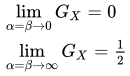
A continuación se muestran los límites con un parámetro finito (distinto de cero) y el otro aproximándose a estos límites:
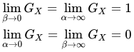
El gráfico adjunto muestra la diferencia entre la media y la media geométrica para los parámetros de forma α y β desde cero hasta 2. Además de que la diferencia entre ellas tiende a cero cuando α y β tienden a infinito y que se vuelve grande para valores de α y β que se aproximan a cero, se puede observar una asimetría evidente de la media geométrica con respecto a los parámetros de forma α y β . La diferencia entre la media geométrica y la media es mayor para valores pequeños de α en relación con β que cuando se intercambian las magnitudes de β y α .
NLJohnson y S. Kotz [ 1 ] sugieren la aproximación logarítmica a la función digamma ψ ( α ) ≈ ln( α − 1/2) que resulta en la siguiente aproximación a la media geométrica:
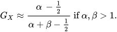
Los valores numéricos para el error relativo en esta aproximación son los siguientes: [ ( α = β = 1): 9,39 % ]; [ ( α = β =2): 1,29% ]; [ ( α = 2, β = 3): 1,51% ]; [ ( α = 3, β = 2): 0,44% ]; [ ( α = β = 3): 0,51% ]; [ ( α = β = 4): 0,26% ]; [ ( α = 3, β = 4): 0,55% ]; [ ( α = 4, β = 3): 0,24% ].
De manera similar, se puede calcular el valor de los parámetros de forma necesarios para que la media geométrica sea igual a 1/2. Dado el valor del parámetro β , ¿cuál sería el valor del otro parámetro, α , necesario para que la media geométrica sea igual a 1/2? La respuesta es que (para β > 1 ), el valor de α requerido tiende hacia β + 1/2 cuando β → ∞ . Por ejemplo, todas estas parejas tienen la misma media geométrica de 1/2: [ β = 1, α = 1.4427 ], [ β = 2, α = 2.46958 ], [ β = 3, α = 3.47943 ], [ β = 4, α = 4.48449 ], [ β = 5, α = 5,48756 ], [ β = 10, α = 10,4938 ], [ β = 100, α = 100,499 ].
La propiedad fundamental de la media geométrica, que puede demostrarse que es falsa para cualquier otra media, es

Esto hace que la media geométrica sea la única media correcta al promediar resultados normalizados , es decir, resultados que se presentan como razones respecto a valores de referencia. [ 13 ] Esto es relevante porque la distribución beta es un modelo adecuado para el comportamiento aleatorio de los porcentajes y es particularmente adecuada para el modelado estadístico de proporciones. La media geométrica juega un papel central en la estimación de máxima verosimilitud, véase la sección "Estimación de parámetros, máxima verosimilitud". De hecho, al realizar la estimación de máxima verosimilitud, además de la media geométrica G X basada en la variable aleatoria X, también aparece naturalmente otra media geométrica: la media geométrica basada en la transformación lineal –– (1 − X ) , la imagen especular de X , denotada por G (1− X ) :
![{\displaystyle G_{1-X}=e^{\operatorname {E} [\ln(1-X)]}=e^{\psi (\beta )-\psi (\alpha +\beta )}}](https://wikimedia.org/api/rest_v1/media/math/render/svg/58d36e067302e87f85db3f0fb1e2902201e38d76)
A lo largo de una línea α = β , se aplican los siguientes límites:

A continuación se muestran los límites con un parámetro finito (distinto de cero) y el otro aproximándose a estos límites:
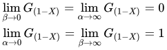
Tiene el siguiente valor aproximado:
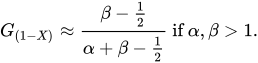
Aunque tanto G X como G 1− X son asimétricos, en el caso de que ambos parámetros de forma sean iguales α = β , las medias geométricas son iguales: G X = G (1− X ) . Esta igualdad se deduce de la siguiente simetría que se muestra entre ambas medias geométricas:

Media armónica


El inverso de la media armónica ( H X ) de una distribución con variable aleatoria X es la media aritmética de 1/ X , o, equivalentemente, su valor esperado. Por lo tanto, la media armónica ( H X ) de una distribución beta con parámetros de forma α y β es:
![{\displaystyle {\begin{aligned}H_{X}&={\frac {1}{\operatorname {E} \left[{\frac {1}{X}}\right]}}\\&={\frac {1}{\int _{0}^{1}{\frac {f(x;\alpha ,\beta )}{x}}\,dx}}\\&={\frac {1}{\int _{0}^{1}{\frac {x^{\alpha -1}(1-x)^{\beta -1}}{x\mathrm {B} (\alpha ,\beta )}}\,dx}}\\&={\frac {\alpha -1}{\alpha +\beta -1}}{\text{ if }}\alpha >1{\text{ and }}\beta >0\\\end{aligned}}}](https://wikimedia.org/api/rest_v1/media/math/render/svg/ed7d99dd7493b9c085cd5d407861730e2a2abf6c)
La media armónica ( H X ) de una distribución beta con α < 1 no está definida, porque su expresión definitoria no está acotada en [0, 1] para un parámetro de forma α menor que la unidad.
Haciendo α = β en la expresión anterior se obtiene
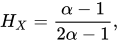
mostrando que para α = β la media armónica varía de 0, para α = β = 1, a 1/2, para α = β → ∞.
A continuación se muestran los límites con un parámetro finito (distinto de cero) y el otro aproximándose a estos límites:
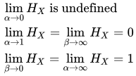
La media armónica desempeña un papel en la estimación de máxima verosimilitud para el caso de cuatro parámetros, además de la media geométrica. De hecho, al realizar la estimación de máxima verosimilitud para el caso de cuatro parámetros, además de la media armónica H X basada en la variable aleatoria X , también aparece naturalmente otra media armónica: la media armónica basada en la transformación lineal (1 − X ), la imagen especular de X , denotada por H 1 − X :
![{\displaystyle H_{1-X}={\frac {1}{\operatorname {E} \left[{\frac {1}{1-X}}\right]}}={\frac {\beta -1}{\alpha +\beta -1}}{\text{ if }}\beta >1,{\text{ and }}\alpha >0.}](https://wikimedia.org/api/rest_v1/media/math/render/svg/48f4fd69f20c4259cb8a50e754df8dfed5a1ddca)
La media armónica ( H (1 − X ) ) de una distribución beta con β < 1 no está definida, porque su expresión definitoria no está acotada en [0, 1] para un parámetro de forma β menor que la unidad.
Haciendo α = β en la expresión anterior se obtiene
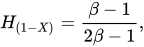
mostrando que para α = β la media armónica varía de 0, para α = β = 1, a 1/2, para α = β → ∞.
A continuación se muestran los límites con un parámetro finito (distinto de cero) y el otro aproximándose a estos límites:
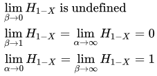
Aunque tanto H X como H 1− X son asimétricos, en el caso de que ambos parámetros de forma sean iguales α = β , las medias armónicas son iguales: H X = H 1− X. Esta igualdad se deduce de la siguiente simetría que se muestra entre ambas medias armónicas:

Medidas de dispersión estadística
Diferencia
La varianza (el segundo momento centrado en la media) de una variable aleatoria X con distribución beta y parámetros α y β es: [ 1 ] [ 14 ]
![{\displaystyle \operatorname {var} (X)=\operatorname {E} \left[(X-\mu )^{2}\right]={\frac {\alpha \beta }{\left(\alpha +\beta \right)^{2}\left(\alpha +\beta +1\right)}}}](https://wikimedia.org/api/rest_v1/media/math/render/svg/d7d2effe47b57f9a004264ee6aac04029d3954de)
Haciendo α = β en la expresión anterior se obtiene
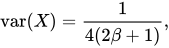
demostrando que para α = β la varianza disminuye monótonamente a medida que α = β aumenta. Haciendo α = β = 0 en esta expresión, se encuentra la varianza máxima var( X ) = 1/4 [ 1 ] que solo ocurre al aproximarse al límite, en α = β = 0 .
La distribución beta también puede parametrizarse en términos de su media μ (0 < μ < 1) y tamaño de muestra ν = α + β ( ν > 0 ) (véase la subsección Media y tamaño de muestra ):

Utilizando esta parametrización , se puede expresar la varianza en términos de la media μ y el tamaño de la muestra ν de la siguiente manera:
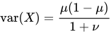
Dado que ν = α + β > 0 , se deduce que var( X ) < μ (1 − μ ) .
Para una distribución simétrica, la media se encuentra en el punto medio de la distribución, μ = 1/2 , y por lo tanto:
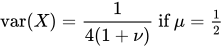
Además, a partir de las expresiones anteriores se pueden obtener los siguientes límites (con solo la variable indicada aproximándose al límite):


Varianza y covarianza geométrica


El logaritmo de la varianza geométrica, ln(var GX ), de una distribución con variable aleatoria X es el segundo momento del logaritmo de X centrado en la media geométrica de X , ln( G X ):
![{\displaystyle {\begin{aligned}\ln \operatorname {var} _{GX}&=\operatorname {E} \left[\left(\ln X-\ln G_{X}\right)^{2}\right]\\&=\operatorname {E} \left[\left(\ln X-\operatorname {E} \left[\ln X\right]\right)^{2}\right]\\&=\operatorname {E} \left[\left(\ln X\right)^{2}\right]-\left(\operatorname {E} [\ln X]\right)^{2}\\&=\operatorname {var} [\ln X]\end{aligned}}}](https://wikimedia.org/api/rest_v1/media/math/render/svg/03642aabe02f83fe6e01e5a136c245d82b898904)
y por lo tanto, la varianza geométrica es:
![{\displaystyle \operatorname {var} _{GX}=e^{\operatorname {var} [\ln X]}}](https://wikimedia.org/api/rest_v1/media/math/render/svg/524cf664ccfd5eb381fd1987926209f1c401a200)
En la matriz de información de Fisher y la curvatura de la función de verosimilitud logarítmica, aparecen el logaritmo de la varianza geométrica de la variable reflejada 1 − X y el logaritmo de la covarianza geométrica entre X y 1 − X :
![{\displaystyle {\begin{aligned}\ln \operatorname {var_{G(1-X)}} &=\operatorname {E} \left[\left(\ln(1-X)-\ln G_{1-X}\right)^{2}\right]\\&=\operatorname {E} \left[\left(\ln(1-X)-\operatorname {E} [\ln(1-X)]\right)^{2}\right]\\&=\operatorname {E} \left[(\ln(1-X))^{2}\right]-\left(\operatorname {E} [\ln(1-X)]\right)^{2}\\&=\operatorname {var} [\ln(1-X)]\\&\\\operatorname {var_{G(1-X)}} &=e^{\operatorname {var} [\ln(1-X)]}\\&\\\ln \operatorname {cov_{G{X,1-X}}} &=\operatorname {E} [(\ln X-\ln G_{X})(\ln(1-X)-\ln G_{1-X})]\\&=\operatorname {E} [(\ln X-\operatorname {E} [\ln X])(\ln(1-X)-\operatorname {E} [\ln(1-X)])]\\&=\operatorname {E} \left[\ln X\ln(1-X)\right]-\operatorname {E} [\ln X]\operatorname {E} [\ln(1-X)]\\&=\operatorname {cov} [\ln X,\ln(1-X)]\\&\\\operatorname {cov} _{G{X,(1-X)}}&=e^{\operatorname {cov} [\ln X,\ln(1-X)]}\end{aligned}}}](https://wikimedia.org/api/rest_v1/media/math/render/svg/657c11ca41846366cb8d9843536af9e002ea4cdf)
Para una distribución beta, los momentos logarítmicos de orden superior pueden derivarse utilizando la representación de una distribución beta como una proporción de dos distribuciones gamma y derivando a través de la integral. Pueden expresarse en términos de funciones poligamma de orden superior. Véase la sección § Momentos de variables aleatorias transformadas logarítmicamente . La varianza de las variables logarítmicas y la covarianza de ln X y ln(1− X ) son:
![{\displaystyle \operatorname {var} [\ln X]=\psi _{1}(\alpha )-\psi _{1}(\alpha +\beta )}](https://wikimedia.org/api/rest_v1/media/math/render/svg/e396e8700267735eb741f73e8906445579c43bc6)
![{\displaystyle \operatorname {var} [\ln(1-X)]=\psi _{1}(\beta )-\psi _{1}(\alpha +\beta )}](https://wikimedia.org/api/rest_v1/media/math/render/svg/70eefadef46c7d56cc13c8221aa3df1d71596b7f)
![{\displaystyle \operatorname {cov} [\ln X,\ln(1-X)]=-\psi _{1}(\alpha +\beta )}](https://wikimedia.org/api/rest_v1/media/math/render/svg/e7a515ada0b9d62c5a3a7b35662b03256d66e3b9)
donde la función trigamma , denotada ψ 1 ( α ), es la segunda de las funciones poligamma , y se define como la derivada de la función digamma :
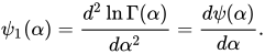
Por lo tanto,
![{\displaystyle \ln \operatorname {var} _{GX}=\operatorname {var} [\ln X]=\psi _{1}(\alpha )-\psi _{1}(\alpha +\beta )}](https://wikimedia.org/api/rest_v1/media/math/render/svg/194b00552edda5d8d026a24872cdb27b604516c9)
![{\displaystyle \ln \operatorname {var} _{G(1-X)}=\operatorname {var} [\ln(1-X)]=\psi _{1}(\beta )-\psi _{1}(\alpha +\beta )}](https://wikimedia.org/api/rest_v1/media/math/render/svg/96dd82553307c025c84da68a3c373aad7467abd2)
![{\displaystyle \ln \operatorname {cov} _{GX,1-X}=\operatorname {cov} [\ln X,\ln(1-X)]=-\psi _{1}(\alpha +\beta )}](https://wikimedia.org/api/rest_v1/media/math/render/svg/40a793c0271e457f671edb0668edc15bbae8740f)
Los gráficos adjuntos muestran las varianzas geométricas logarítmicas y la covarianza geométrica logarítmica en función de los parámetros de forma α y β . Los gráficos muestran que las varianzas geométricas logarítmicas y la covarianza geométrica logarítmica son cercanas a cero para parámetros de forma α y β mayores que 2, y que las varianzas geométricas logarítmicas aumentan rápidamente para valores de parámetros de forma α y β menores que la unidad. Las varianzas geométricas logarítmicas son positivas para todos los valores de los parámetros de forma. La covarianza geométrica logarítmica es negativa para todos los valores de los parámetros de forma, y alcanza valores negativos elevados para α y β menores que la unidad.
A continuación se muestran los límites con un parámetro finito (distinto de cero) y el otro aproximándose a estos límites:

Límites con dos parámetros variables:

Aunque tanto ln(var GX ) como ln(var G (1 − X ) ) son asimétricos, cuando los parámetros de forma son iguales, α = β , se tiene: ln(var GX ) = ln(var G (1− X ) ). Esta igualdad se deriva de la siguiente simetría que se muestra entre ambas varianzas geométricas logarítmicas:

La covarianza geométrica logarítmica es simétrica:

Desviación absoluta media alrededor de la media


La desviación absoluta media alrededor de la media para la distribución beta con parámetros de forma α y β es: [ 9 ]
![{\displaystyle \operatorname {E} [|X-E[X]|]={\frac {2\alpha ^{\alpha }\beta ^{\beta }}{\mathrm {B} (\alpha ,\beta )(\alpha +\beta )^{\alpha +\beta +1}}}}](https://wikimedia.org/api/rest_v1/media/math/render/svg/6d1c6330a91df22b40cedc7903dbc70120d66cf9)
La desviación absoluta media alrededor de la media es un estimador más robusto de la dispersión estadística que la desviación estándar para distribuciones beta con colas y puntos de inflexión a cada lado de la moda, distribuciones Beta( α , β ) con α , β > 2, ya que depende de las desviaciones lineales (absolutas) en lugar de las desviaciones cuadráticas respecto a la media. Por lo tanto, el efecto de desviaciones muy grandes respecto a la media no se ve tan sobrevalorado.
Utilizando la aproximación de Stirling a la función Gamma , NLJohnson y S.Kotz [ 1 ] derivaron la siguiente aproximación para valores de los parámetros de forma mayores que la unidad (el error relativo para esta aproximación es solo −3,5% para α = β = 1, y disminuye a cero cuando α → ∞, β → ∞):
![{\displaystyle {\begin{aligned}{\frac {\text{mean abs. dev. from mean}}{\text{standard deviation}}}&={\frac {\operatorname {E} [|X-E[X]|]}{\sqrt {\operatorname {var} (X)}}}\\&\approx {\sqrt {\frac {2}{\pi }}}\left(1+{\frac {7}{12(\alpha +\beta )}}{}-{\frac {1}{12\alpha }}-{\frac {1}{12\beta }}\right),{\text{ if }}\alpha ,\beta >1.\end{aligned}}}](https://wikimedia.org/api/rest_v1/media/math/render/svg/c196a5a2eb110b71471a3dc019241c6cb8c3f927)
En el límite α → ∞, β → ∞, la razón entre la desviación absoluta media y la desviación estándar (para la distribución beta) se vuelve igual a la razón de las mismas medidas para la distribución normal:. Para α = β = 1 esta razón es igual a, de modo que desde α = β = 1 hasta α , β → ∞ la razón disminuye en un 8,5%. Para α = β = 0 la desviación estándar es exactamente igual a la desviación absoluta media alrededor de la media. Por lo tanto, esta razón disminuye en un 15% desde α = β = 0 hasta α = β = 1, y en un 25% desde α = β = 0 hasta α , β → ∞ . Sin embargo, para distribuciones beta asimétricas tales que α → 0 o β → 0, la razón de la desviación estándar a la desviación absoluta media tiende a infinito (aunque cada una de ellas, individualmente, tiende a cero) porque la desviación absoluta media tiende a cero más rápido que la desviación estándar.


Utilizando la parametrización en términos de media μ y tamaño de muestra ν = α + β > 0:
La desviación absoluta media alrededor de la media se puede expresar en términos de la media μ y el tamaño de la muestra ν de la siguiente manera:
![{\displaystyle \operatorname {E} [|X-E[X]|]={\frac {2\mu ^{\mu \nu }(1-\mu )^{(1-\mu )\nu }}{\nu \mathrm {B} (\mu \nu ,(1-\mu )\nu )}}}](https://wikimedia.org/api/rest_v1/media/math/render/svg/027efecf8aaefea8c805194e47a1374ffcb63cb8)
Para una distribución simétrica, la media se encuentra en el punto medio de la distribución, μ = 1/2, y por lo tanto:
![{\displaystyle {\begin{aligned}\operatorname {E} [|X-E[X]|]={\frac {2^{1-\nu }}{\nu \mathrm {B} ({\tfrac {\nu }{2}},{\tfrac {\nu }{2}})}}&={\frac {2^{1-\nu }\Gamma (\nu )}{\nu (\Gamma ({\tfrac {\nu }{2}}))^{2}}}\\\lim _{\nu \to 0}\left(\lim _{\mu \to {\frac {1}{2}}}\operatorname {E} [|X-E[X]|]\right)&={\frac {1}{2}}\\\lim _{\nu \to \infty }\left(\lim _{\mu \to {\frac {1}{2}}}\operatorname {E} [|X-E[X]|]\right)&=0\end{aligned}}}](https://wikimedia.org/api/rest_v1/media/math/render/svg/745a053a1ef3cc7edf07332763b401bd09b40e42)
Además, a partir de las expresiones anteriores se pueden obtener los siguientes límites (con solo la variable indicada aproximándose al límite):
![{\displaystyle {\begin{aligned}\lim _{\beta \to 0}\operatorname {E} [|X-E[X]|]&=\lim _{\alpha \to 0}\operatorname {E} [|X-E[X]|]=0\\\lim _{\beta \to \infty }\operatorname {E} [|X-E[X]|]&=\lim _{\alpha \to \infty }\operatorname {E} [|X-E[X]|]=0\\\lim _{\mu \to 0}\operatorname {E} [|X-E[X]|]&=\lim _{\mu \to 1}\operatorname {E} [|X-E[X]|]=0\\\lim _{\nu \to 0}\operatorname {E} [|X-E[X]|]&={\sqrt {\mu (1-\mu )}}\\\lim _{\nu \to \infty }\operatorname {E} [|X-E[X]|]&=0\end{aligned}}}](https://wikimedia.org/api/rest_v1/media/math/render/svg/87c43b4a05f8ea3acf3f15b0a16f6ee07811ac6b)
Diferencia absoluta media
La diferencia absoluta media para la distribución beta es:
![{\displaystyle {\begin{aligned}\mathrm {MD} &=\int _{0}^{1}\int _{0}^{1}f(x;\alpha ,\beta )\,f(y;\alpha ,\beta )\left|x-y\right|dx\,dy\\[1ex]&={\frac {4}{\alpha +\beta }}{\frac {B(\alpha +\beta ,\alpha +\beta )}{B(\alpha ,\alpha )B(\beta ,\beta )}}\end{aligned}}}](https://wikimedia.org/api/rest_v1/media/math/render/svg/0de290eea66b8a424727bff1b9a02f53f2607361)
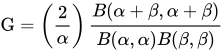
El coeficiente de Gini para la distribución beta es la mitad de la diferencia absoluta media relativa:
Oblicuidad

La asimetría (el tercer momento centrado en la media, normalizado por la potencia 3/2 de la varianza) de la distribución beta es [ 1 ]
![{\displaystyle \gamma _{1}={\frac {\operatorname {E} \left[\left(X-\mu \right)^{3}\right]}{\left(\operatorname {var} (X)\right)^{3/2}}}={\frac {2\left(\beta -\alpha \right){\sqrt {\alpha +\beta +1}}}{\left(\alpha +\beta +2\right){\sqrt {\alpha \beta }}}}.}](https://wikimedia.org/api/rest_v1/media/math/render/svg/1c880f0b8322d91fe382f87eaa4f8730faa164ed)
Si hacemos α = β en la expresión anterior, obtenemos γ 1 = 0, lo que demuestra una vez más que para α = β la distribución es simétrica y, por lo tanto, la asimetría es cero. Asimetría positiva (cola derecha) para α < β , asimetría negativa (cola izquierda) para α > β .
Utilizando la parametrización en términos de media μ y tamaño de muestra ν = α + β :
La asimetría se puede expresar en términos de la media μ y el tamaño de la muestra ν de la siguiente manera:
![{\displaystyle \gamma _{1}={\frac {\operatorname {E} [(X-\mu )^{3}]}{\left(\operatorname {var} (X)\right)^{3/2}}}={\frac {2(1-2\mu ){\sqrt {1+\nu }}}{(2+\nu ){\sqrt {\mu (1-\mu )}}}}.}](https://wikimedia.org/api/rest_v1/media/math/render/svg/c88399efb587f7d2443ddb232e4b24f2763050b9)
La asimetría también puede expresarse simplemente en términos de la varianza var y la media μ de la siguiente manera:
![{\displaystyle \gamma _{1}={\frac {\operatorname {E} [(X-\mu )^{3}]}{(\operatorname {var} (X))^{3/2}}}={\frac {2(1-2\mu ){\sqrt {\operatorname {var} }}}{\mu (1-\mu )+\operatorname {var} }}{\text{ if }}\operatorname {var} <\mu (1-\mu )}](https://wikimedia.org/api/rest_v1/media/math/render/svg/6b48373ac7ce8096381e7f74edf9e44bc435ad13)
El gráfico adjunto de asimetría en función de la varianza y la media muestra que la varianza máxima (1/4) está relacionada con la asimetría cero y la condición de simetría ( μ = 1/2), y que la asimetría máxima (infinito positivo o negativo) se produce cuando la media se sitúa en un extremo o en el otro, de modo que la "masa" de la distribución de probabilidad se concentra en los extremos (varianza mínima).
La siguiente expresión para el cuadrado de la asimetría, en términos del tamaño de la muestra ν = α + β y la varianza var, es útil para la estimación de cuatro parámetros mediante el método de los momentos:
![{\displaystyle (\gamma _{1})^{2}={\frac {\left(\operatorname {E} [(X-\mu )^{3}]\right)^{2}}{\left(\operatorname {var} (X)\right)^{3}}}={\frac {4}{(2+\nu )^{2}}}\left({\frac {1}{\operatorname {var} }}-4(1+\nu )\right)}](https://wikimedia.org/api/rest_v1/media/math/render/svg/b4f7b7d9a6d73e9bbcc43812b8f3fd573bc02ee3)
Esta expresión da correctamente una asimetría de cero para α = β , ya que en ese caso (véase § Varianza ):.

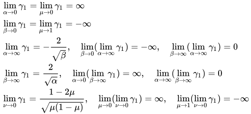
Para el caso simétrico ( α = β ), la asimetría es igual a 0 en todo el rango, y se aplican los siguientes límites:

Para los casos asimétricos ( α ≠ β ) se pueden obtener los siguientes límites (con solo la variable indicada aproximándose al límite) a partir de las expresiones anteriores:


Curtosis

La distribución beta se ha aplicado en el análisis acústico para evaluar daños en engranajes, ya que se ha informado que la curtosis de la distribución beta es un buen indicador del estado de un engranaje. [ 15 ] La curtosis también se ha utilizado para distinguir la señal sísmica generada por los pasos de una persona de otras señales. Como las personas u otros objetivos que se mueven en el suelo generan señales continuas en forma de ondas sísmicas, se pueden separar diferentes objetivos en función de las ondas sísmicas que generan. La curtosis es sensible a las señales impulsivas, por lo que es mucho más sensible a la señal generada por los pasos humanos que a otras señales generadas por vehículos, viento, ruido, etc. [ 16 ] Desafortunadamente, la notación para la curtosis no se ha estandarizado. Kenney y Keeping [ 17 ] utilizan el símbolo γ 2 para la curtosis de exceso , pero Abramowitz y Stegun [ 18 ] utilizan una terminología diferente. Para evitar confusiones [ 19 ] entre la curtosis (el cuarto momento centrado en la media, normalizado por el cuadrado de la varianza) y el exceso de curtosis, cuando se utilicen símbolos, se deletrearán de la siguiente manera: [ 9 ] [ 20 ]
![{\displaystyle {\begin{aligned}{\text{excess kurtosis}}&={\text{kurtosis}}-3\\&={\frac {\operatorname {E} [(X-\mu )^{4}]}{(\operatorname {var} (X))^{2}}}-3\\&={\frac {6[\alpha ^{3}-\alpha ^{2}(2\beta -1)+\beta ^{2}(\beta +1)-2\alpha \beta (\beta +2)]}{\alpha \beta (\alpha +\beta +2)(\alpha +\beta +3)}}\\&={\frac {6[(\alpha -\beta )^{2}(\alpha +\beta +1)-\alpha \beta (\alpha +\beta +2)]}{\alpha \beta (\alpha +\beta +2)(\alpha +\beta +3)}}.\end{aligned}}}](https://wikimedia.org/api/rest_v1/media/math/render/svg/ed8320d4f38ba9260f8ad91c30238abc08306dc8)
Haciendo α = β en la expresión anterior se obtiene

Por lo tanto, para las distribuciones beta simétricas, la curtosis en exceso es negativa, aumentando desde un valor mínimo de −2 en el límite cuando { α = β } → 0, y aproximándose a un valor máximo de cero cuando { α = β } → ∞. El valor de −2 es el valor mínimo de curtosis en exceso que cualquier distribución (no solo las distribuciones beta, sino cualquier distribución de cualquier tipo posible) puede alcanzar. Este valor mínimo se alcanza cuando toda la densidad de probabilidad se concentra completamente en cada extremo x = 0 y x = 1, sin nada en el medio: una distribución de Bernoulli de 2 puntos con igual probabilidad 1/2 en cada extremo (un lanzamiento de moneda: véase la sección siguiente "Curtosis limitada por el cuadrado de la asimetría" para más detalles). La descripción de la curtosis como una medida de los "valores atípicos potenciales" (o "valores extremos raros potenciales") de la distribución de probabilidad es correcta para todas las distribuciones, incluida la distribución beta. Cuando se presentan valores extremos poco frecuentes en la distribución beta, mayor es su curtosis; de lo contrario, la curtosis es menor. Para α ≠ β , en distribuciones beta asimétricas, la curtosis en exceso puede alcanzar valores positivos ilimitados (particularmente para α → 0 para β finito , o para β → 0 para α finito ) debido a que el lado opuesto a la moda producirá valores extremos ocasionales. La curtosis mínima se produce cuando la densidad de masa se concentra por igual en cada extremo (y, por lo tanto, la media se encuentra en el centro), y no existe densidad de masa de probabilidad entre los extremos.
Utilizando la parametrización en términos de media μ y tamaño de muestra ν = α + β :

La curtosis en exceso se puede expresar en términos de la media μ y el tamaño de la muestra ν de la siguiente manera:

La curtosis en exceso también puede expresarse en términos de los siguientes dos parámetros: la varianza var y el tamaño de la muestra ν, de la siguiente manera:

y, en términos de la varianza var y la media μ, de la siguiente manera:

La gráfica de la curtosis en exceso en función de la varianza y la media muestra que el valor mínimo de la curtosis en exceso (−2, que es el valor mínimo posible para cualquier distribución) está íntimamente ligado al valor máximo de la varianza (1/4) y a la condición de simetría: la media se produce en el punto medio ( μ = 1/2). Esto ocurre para el caso simétrico de α = β = 0, con asimetría cero. En el límite, esta es la distribución de Bernoulli de 2 puntos con igual probabilidad 1/2 en cada extremo de la función delta de Dirac x = 0 y x = 1 y probabilidad cero en cualquier otro lugar. (Como lanzar una moneda: una cara de la moneda es x = 0 y la otra es x = 1). La varianza es máxima porque la distribución es bimodal sin nada entre los dos modos (picos) en cada extremo. La curtosis excesiva es mínima: la densidad de probabilidad es cero en la media y se concentra en los dos picos de cada extremo. La curtosis excesiva alcanza el valor mínimo posible (para cualquier distribución) cuando la función de densidad de probabilidad tiene dos picos en cada extremo: es bipico, sin nada entre ellos.
Por otro lado, el gráfico muestra que para los casos de asimetría extrema, donde la media se encuentra cerca de uno u otro extremo ( μ = 0 o μ = 1), la varianza es cercana a cero y la curtosis en exceso se aproxima rápidamente al infinito cuando la media de la distribución se aproxima a cualquiera de los extremos.
Alternativamente, la curtosis en exceso también puede expresarse en términos de los siguientes dos parámetros: el cuadrado de la asimetría y el tamaño de la muestra ν, como sigue:

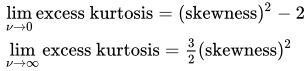
A partir de esta última expresión, se pueden obtener los mismos límites publicados hace más de un siglo por Karl Pearson [ 21 ] para la distribución beta (véase la sección siguiente titulada "Curtosis limitada por el cuadrado de la asimetría"). Haciendo α + β = ν = 0 en la expresión anterior, se obtiene el límite inferior de Pearson (los valores de la asimetría y la curtosis en exceso por debajo del límite ( curtosis en exceso + 2 − asimetría 2 = 0) no pueden darse para ninguna distribución, y por lo tanto Karl Pearson denominó apropiadamente a la región por debajo de este límite la "región imposible"). El límite de α + β = ν → ∞ determina el límite superior de Pearson.
por lo tanto:

Los valores de ν = α + β tales que ν varía de cero a infinito, 0 < ν < ∞, abarcan toda la región de la distribución beta en el plano de curtosis en exceso frente a asimetría al cuadrado.
Para el caso simétrico ( α = β ), se aplican los siguientes límites:
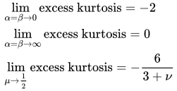
Para los casos asimétricos ( α ≠ β ) se pueden obtener los siguientes límites (con solo la variable indicada aproximándose al límite) a partir de las expresiones anteriores:


Función característica


La función característica es la transformada de Fourier de la función de densidad de probabilidad. La función característica de la distribución beta es la función hipergeométrica confluente de Kummer (de primer tipo): [ 1 ] [ 18 ] [ 22 ]
- ;\beta ;t)&=\operatorname {E} \left[e^{itX}\right]\\&=\int _{0}^{1}e^{itx}f(x;\alpha ,\beta )\,dx\\&={}_{1}F_{1}(\alpha ;\alpha +\beta ;it)\!\\&=\sum _{n=0}^{\infty }{\frac {\alpha ^{\overline {n}}(it)^{n}}{(\alpha +\beta )^{\overline {n}}n!}}\\&=1+\sum _{k=1}^{\infty }\left(\prod _{r=0}^{k-1}{\frac {\alpha +r}{\alpha +\beta +r}}\right){\frac {(it)^{k}}{k!}}\end{aligned}}}
![{\displaystyle {\begin{aligned}\varphi _{X}(\alpha ;\beta ;t)&=\operatorname {E} \left[e^{itX}\right]\\&=\int _{0}^{1}e^{itx}f(x;\alpha ,\beta )\,dx\\&={}_{1}F_{1}(\alpha ;\alpha +\beta ;it)\!\\&=\sum _{n=0}^{\infty }{\frac {\alpha ^{\overline {n}}(it)^{n}}{(\alpha +\beta )^{\overline {n}}n!}}\\&=1+\sum _{k=1}^{\infty }\left(\prod _{r=0}^{k-1}{\frac {\alpha +r}{\alpha +\beta +r}}\right){\frac {(it)^{k}}{k!}}\end{aligned}}}](https://wikimedia.org/api/rest_v1/media/math/render/svg/2e0e8f5d3bf4ec0cbe9b911e26c961e9ebaefdd8)
dónde

es el factorial creciente . El valor de la función característica para t = 0 es uno:
;\beta ;0)={}_{1}F_{1}(\alpha ;\alpha +\beta ;0)=1.}

Además, las partes real e imaginaria de la función característica gozan de las siguientes simetrías con respecto al origen de la variable t :
;\alpha +\beta ;it)\right]=\operatorname {Re} \left[{}_{1}F_{1}(\alpha ;\alpha +\beta ;-it)\right]} ;\alpha +\beta ;it)\right]=-\operatorname {Im} \left[{}_{1}F_{1}(\alpha ;\alpha +\beta ;-it)\right]}
![{\displaystyle \operatorname {Re} \left[{}_{1}F_{1}(\alpha ;\alpha +\beta ;it)\right]=\operatorname {Re} \left[{}_{1}F_{1}(\alpha ;\alpha +\beta ;-it)\right]}](https://wikimedia.org/api/rest_v1/media/math/render/svg/468f2135d76bd1b522c84092679209ff6abd5845)
![{\displaystyle \operatorname {Im} \left[{}_{1}F_{1}(\alpha ;\alpha +\beta ;it)\right]=-\operatorname {Im} \left[{}_{1}F_{1}(\alpha ;\alpha +\beta ;-it)\right]}](https://wikimedia.org/api/rest_v1/media/math/render/svg/0fca8984292cc85cb8a37ecb5a2b7c04b5596282)
El caso simétrico α = β simplifica la función característica de la distribución beta a una función de Bessel , ya que en el caso especial α + β = 2 α la función hipergeométrica confluente (de primera especie) se reduce a una función de Bessel (la función de Bessel modificada de primera especie).) utilizando la segunda transformación de Kummer de la siguiente manera:

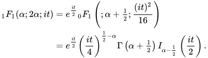
En los gráficos adjuntos, se muestra la parte real (Re) de la función característica de la distribución beta para los casos simétricos ( α = β ) y asimétricos ( α ≠ β ).
Otros momentos
Función generadora de momentos
También se deduce [ 1 ] [ 9 ] que la función generadora de momentos es
;\beta ;t)&=\operatorname {E} \left[e^{tX}\right]\\[4pt]&=\int _{0}^{1}e^{tx}f(x;\alpha ,\beta )\,dx\\[4pt]&={}_{1}F_{1}(\alpha ;\alpha +\beta ;t)\\[4pt]&=\sum _{n=0}^{\infty }{\frac {\alpha ^{\overline {n}}}{(\alpha +\beta )^{\overline {n}}}}{\frac {t^{n}}{n!}}\\[4pt]&=1+\sum _{k=1}^{\infty }\left(\prod _{r=0}^{k-1}{\frac {\alpha +r}{\alpha +\beta +r}}\right){\frac {t^{k}}{k!}}.\end{aligned}}}
![{\displaystyle {\begin{aligned}M_{X}(\alpha ;\beta ;t)&=\operatorname {E} \left[e^{tX}\right]\\[4pt]&=\int _{0}^{1}e^{tx}f(x;\alpha ,\beta )\,dx\\[4pt]&={}_{1}F_{1}(\alpha ;\alpha +\beta ;t)\\[4pt]&=\sum _{n=0}^{\infty }{\frac {\alpha ^{\overline {n}}}{(\alpha +\beta )^{\overline {n}}}}{\frac {t^{n}}{n!}}\\[4pt]&=1+\sum _{k=1}^{\infty }\left(\prod _{r=0}^{k-1}{\frac {\alpha +r}{\alpha +\beta +r}}\right){\frac {t^{k}}{k!}}.\end{aligned}}}](https://wikimedia.org/api/rest_v1/media/math/render/svg/7c5c0eea7bcffadb73fef0c85534a8bdca36ebbb)
En particular MX ( α ; β ; 0) = 1.
Momentos más elevados
Utilizando la función generadora de momentos , el k -ésimo momento bruto viene dado por [ 1 ] el factor
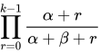
multiplicando el término (de la serie exponencial)en la serie de la función generadora de momentos

![{\displaystyle \operatorname {E} [X^{k}]={\frac {\alpha ^{\overline {k}}}{(\alpha +\beta )^{\overline {k}}}}=\prod _{r=0}^{k-1}{\frac {\alpha +r}{\alpha +\beta +r}}}](https://wikimedia.org/api/rest_v1/media/math/render/svg/af7e0927f7f82eccc61e9fb55883ce96d7f958f1)
donde ( x ) ( k ) es un símbolo de Pochhammer que representa el factorial ascendente. También se puede escribir de forma recursiva como
![{\displaystyle \operatorname {E} [X^{k}]={\frac {\alpha +k-1}{\alpha +\beta +k-1}}\operatorname {E} [X^{k-1}].}](https://wikimedia.org/api/rest_v1/media/math/render/svg/069cb373a905b1e8a5a82a0e3b028e88f63672e2)
Dado que la función generadora de momentos ;\beta ;\cdot )} tiene un radio de convergencia positivo,la distribución beta está determinada por sus momentos . [ 23 ]

Momentos de variables aleatorias transformadas
Momentos de variables aleatorias transformadas linealmente, producto e invertidas
También se pueden mostrar las siguientes expectativas para una variable aleatoria transformada, [ 1 ] donde la variable aleatoria X tiene una distribución Beta con parámetros α y β : X ~ Beta( α , β ). El valor esperado de la variable 1 − X es la simetría especular del valor esperado basado en X :
![{\displaystyle {\begin{aligned}\operatorname {E} [1-X]&={\frac {\beta }{\alpha +\beta }}\\\operatorname {E} [X(1-X)]&=\operatorname {E} [(1-X)X]={\frac {\alpha \beta }{(\alpha +\beta )(\alpha +\beta +1)}}\end{aligned}}}](https://wikimedia.org/api/rest_v1/media/math/render/svg/43fc49b9eafccd56d39c236b26d222dde51638ce)
Debido a la simetría especular de la función de densidad de probabilidad de la distribución beta, las varianzas basadas en las variables X y 1 − X son idénticas, y la covarianza en X (1 − X ) es el negativo de la varianza:
![{\displaystyle \operatorname {var} [(1-X)]=\operatorname {var} [X]=-\operatorname {cov} [X,(1-X)]={\frac {\alpha \beta }{(\alpha +\beta )^{2}(\alpha +\beta +1)}}}](https://wikimedia.org/api/rest_v1/media/math/render/svg/7273cc84a6c789724b985c34059fa75a62bce631)
Estos son los valores esperados para las variables invertidas (estos están relacionados con las medias armónicas, véase § Media armónica ):
![{\displaystyle {\begin{aligned}\operatorname {E} \left[{\frac {1}{X}}\right]&={\frac {\alpha +\beta -1}{\alpha -1}}&&{\text{ if }}\alpha >1\\\operatorname {E} \left[{\frac {1}{1-X}}\right]&={\frac {\alpha +\beta -1}{\beta -1}}&&{\text{ if }}\beta >1\end{aligned}}}](https://wikimedia.org/api/rest_v1/media/math/render/svg/972a9c1853e6991aac6666b06c0a633a0caad5b7)
La siguiente transformación, al dividir la variable X por su imagen especular X /(1 − X )), da como resultado el valor esperado de la "distribución beta invertida" o distribución beta prima (también conocida como distribución beta de segundo tipo o tipo VI de Pearson ): [ 1 ]
![{\displaystyle {\begin{aligned}\operatorname {E} \left[{\frac {X}{1-X}}\right]&={\frac {\alpha }{\beta -1}}&&{\text{ if }}\beta >1\\\operatorname {E} \left[{\frac {1-X}{X}}\right]&={\frac {\beta }{\alpha -1}}&&{\text{ if }}\alpha >1\end{aligned}}}](https://wikimedia.org/api/rest_v1/media/math/render/svg/db2a0928a7f906bcbe5cfd9d0c57713c9ab5cfb7)
Las varianzas de estas variables transformadas se pueden obtener mediante integración, como los valores esperados de los segundos momentos centrados en las variables correspondientes:
![{\displaystyle {\begin{aligned}\operatorname {var} \left[{\frac {1}{X}}\right]&=\operatorname {E} \left[\left({\frac {1}{X}}-\operatorname {E} \left[{\frac {1}{X}}\right]\right)^{2}\right]=\operatorname {var} \left[{\frac {1-X}{X}}\right]\\&=\operatorname {E} \left[\left({\frac {1-X}{X}}-\operatorname {E} \left[{\frac {1-X}{X}}\right]\right)^{2}\right]={\frac {\beta (\alpha +\beta -1)}{\left(\alpha -2\right)\left(\alpha -1\right)^{2}}}{\text{ if }}\alpha >2\end{aligned}}}](https://wikimedia.org/api/rest_v1/media/math/render/svg/ab8c3db5d04798c92c6360624060ba583ebdf3df)
La siguiente varianza de la variable X dividida por su imagen especular ( X /(1− X ) da como resultado la varianza de la "distribución beta invertida" o distribución beta prima (también conocida como distribución beta de segundo tipo o tipo VI de Pearson ): [ 1 ]
![{\displaystyle {\begin{aligned}\operatorname {var} \left[{\frac {1}{1-X}}\right]&=\operatorname {E} \left[\left({\frac {1}{1-X}}-\operatorname {E} \left[{\frac {1}{1-X}}\right]\right)^{2}\right]=\operatorname {var} \left[{\frac {X}{1-X}}\right]\\[1ex]&=\operatorname {E} \left[\left({\frac {X}{1-X}}-\operatorname {E} \left[{\frac {X}{1-X}}\right]\right)^{2}\right]={\frac {\alpha (\alpha +\beta -1)}{\left(\beta -2\right)\left(\beta -1\right)^{2}}}{\text{ if }}\beta >2\end{aligned}}}](https://wikimedia.org/api/rest_v1/media/math/render/svg/76d83000746ff4852e63b063948f9db8110d2d22)
Las covarianzas son:
Estas expectativas y varianzas aparecen en la matriz de información de Fisher de cuatro parámetros ( § Información de Fisher .)
![{\displaystyle {\begin{aligned}\operatorname {cov} \left[{\frac {1}{X}},{\frac {1}{1-X}}\right]&=\operatorname {cov} \left[{\frac {1-X}{X}},{\frac {X}{1-X}}\right]=\operatorname {cov} \left[{\frac {1}{X}},{\frac {X}{1-X}}\right]\\[1ex]&=\operatorname {cov} \left[{\frac {1-X}{X}},{\frac {1}{1-X}}\right]={\frac {\alpha +\beta -1}{(\alpha -1)(\beta -1)}}{\text{ if }}\alpha ,\beta >1\end{aligned}}}](https://wikimedia.org/api/rest_v1/media/math/render/svg/ce6ebb40e9f206c0269353799307092c2edbcfa0)
Momentos de variables aleatorias transformadas logarítmicamente

En esta sección se analizan los valores esperados para las transformaciones logarítmicas (útiles para las estimaciones de máxima verosimilitud ; véase § Estimación de parámetros, Máxima verosimilitud ). Las siguientes transformaciones lineales logarítmicas están relacionadas con las medias geométricas G X y G 1− X (véase § Media geométrica ):
![{\displaystyle {\begin{aligned}\operatorname {E} [\ln X]&=\psi (\alpha )-\psi (\alpha +\beta )=-\operatorname {E} \left[\ln {\frac {1}{X}}\right],\\\operatorname {E} [\ln(1-X)]&=\psi (\beta )-\psi (\alpha +\beta )=-\operatorname {E} \left[\ln {\frac {1}{1-X}}\right].\end{aligned}}}](https://wikimedia.org/api/rest_v1/media/math/render/svg/af6c3188ac96160054472db2a23bab9a22f1e486)
Donde la función digamma ψ ( α ) se define como la derivada logarítmica de la función gamma : [ 18 ]

Las transformaciones logit son interesantes, [ 24 ] ya que suelen transformar varias formas (incluidas las formas de J) en densidades en forma de campana (generalmente sesgadas) sobre la variable logit, y pueden eliminar las singularidades de los extremos sobre la variable original:
![{\displaystyle {\begin{aligned}\operatorname {E} \left[\ln {\frac {X}{1-X}}\right]&=\psi (\alpha )-\psi (\beta )=\operatorname {E} [\ln X]+\operatorname {E} \left[\ln {\frac {1}{1-X}}\right],\\\operatorname {E} \left[\ln {\frac {1-X}{X}}\right]&=\psi (\beta )-\psi (\alpha )=-\operatorname {E} \left[\ln {\frac {X}{1-X}}\right].\end{aligned}}}](https://wikimedia.org/api/rest_v1/media/math/render/svg/a30b0fbbefff93de41d6775f2ab623670f09a4b2)
Johnson [ 25 ] consideró la distribución de la variable transformada logit ln( X /1 − X ), incluyendo su función generadora de momentos y aproximaciones para valores grandes de los parámetros de forma. Esta transformación extiende el soporte finito [0, 1] basado en la variable original X a un soporte infinito en ambas direcciones de la recta real (−∞, +∞). El logit de una variable beta tiene la distribución logística beta .
Los momentos logarítmicos de orden superior se pueden obtener utilizando la representación de una distribución beta como una proporción de dos distribuciones gamma y derivando a través de la integral. Se pueden expresar en términos de funciones poligamma de orden superior de la siguiente manera:
![{\displaystyle {\begin{aligned}\operatorname {E} \left[\ln ^{2}(X)\right]&=(\psi (\alpha )-\psi (\alpha +\beta ))^{2}+\psi _{1}(\alpha )-\psi _{1}(\alpha +\beta ),\\\operatorname {E} \left[\ln ^{2}(1-X)\right]&=(\psi (\beta )-\psi (\alpha +\beta ))^{2}+\psi _{1}(\beta )-\psi _{1}(\alpha +\beta ),\\\operatorname {E} \left[\ln(X)\ln(1-X)\right]&=(\psi (\alpha )-\psi (\alpha +\beta ))(\psi (\beta )-\psi (\alpha +\beta ))-\psi _{1}(\alpha +\beta ).\end{aligned}}}](https://wikimedia.org/api/rest_v1/media/math/render/svg/b42eb1276e349df39df3051df11e0e16afe88e2e)
Por lo tanto, la varianza de las variables logarítmicas y la covarianza de ln( X ) y ln(1− X ) son:
![{\displaystyle {\begin{aligned}\operatorname {cov} [\ln X,\ln(1-X)]&=\operatorname {E} \left[\ln X\ln(1-X)\right]-\operatorname {E} [\ln X]\operatorname {E} [\ln(1-X)]\\&=-\psi _{1}(\alpha +\beta )\\&\\\operatorname {var} [\ln X]&=\operatorname {E} [\ln ^{2}X]-(\operatorname {E} [\ln X])^{2}\\&=\psi _{1}(\alpha )-\psi _{1}(\alpha +\beta )\\&=\psi _{1}(\alpha )+\operatorname {cov} [\ln X,\ln(1-X)]\\&\\\operatorname {var} [\ln(1-X)]&=\operatorname {E} [\ln ^{2}(1-X)]-(\operatorname {E} [\ln(1-X)])^{2}\\&=\psi _{1}(\beta )-\psi _{1}(\alpha +\beta )\\&=\psi _{1}(\beta )+\operatorname {cov} [\ln X,\ln(1-X)]\end{aligned}}}](https://wikimedia.org/api/rest_v1/media/math/render/svg/53f5f8222528ab3aa1e5f610f49d440d348f7d40)
donde la función trigamma , denotada ψ 1 ( α ), es la segunda de las funciones poligamma , y se define como la derivada de la función digamma :
Las varianzas y covarianzas de las variables transformadas logarítmicamente X y (1 − X ) son diferentes, en general, porque la transformación logarítmica destruye la simetría especular de las variables originales X y (1 − X ), ya que el logaritmo se aproxima a menos infinito para la variable que se aproxima a cero.
Estas varianzas y covarianzas logarítmicas son los elementos de la matriz de información de Fisher para la distribución beta. También son una medida de la curvatura de la función de verosimilitud logarítmica (véase la sección sobre estimación de máxima verosimilitud).
Las varianzas de las variables logarítmicas inversas son idénticas a las varianzas de las variables logarítmicas:
![{\displaystyle {\begin{aligned}\operatorname {var} \left[\ln {\frac {1}{X}}\right]&=\operatorname {var} [\ln X]=\psi _{1}(\alpha )-\psi _{1}(\alpha +\beta ),\\\operatorname {var} \left[\ln {\frac {1}{1-X}}\right]&=\operatorname {var} [\ln(1-X)]=\psi _{1}(\beta )-\psi _{1}(\alpha +\beta ),\\\operatorname {cov} \left[\ln {\frac {1}{X}},\,\ln {\frac {1}{1-X}}\right]&=\operatorname {cov} [\ln X,\ln(1-X)]=-\psi _{1}(\alpha +\beta ).\end{aligned}}}](https://wikimedia.org/api/rest_v1/media/math/render/svg/18739db82ac6e431571537bb8f09ff006d670b04)
También se deduce que las varianzas de las variables transformadas mediante logit son
![{\displaystyle {\begin{aligned}\operatorname {var} \left[\ln {\frac {X}{1-X}}\right]&=\operatorname {var} \left[\ln {\frac {1-X}{X}}\right]\\&=-\operatorname {cov} \left[\ln {\frac {X}{1-X}},\,\ln {\frac {1-X}{X}}\right]\\[1ex]&=\psi _{1}(\alpha )+\psi _{1}(\beta ).\end{aligned}}}](https://wikimedia.org/api/rest_v1/media/math/render/svg/b0f473b85a33bfd20c16bd2e752af80def37388a)
Cantidades de información (entropía)
Dada una variable aleatoria con distribución beta, X ~ Beta( α , β ), la entropía diferencial de X es (medida en nats ), [ 26 ] el valor esperado del negativo del logaritmo de la función de densidad de probabilidad :
![{\displaystyle {\begin{aligned}h(X)&=\operatorname {E} \left[-\ln f(X;\alpha ,\beta )\right]\\[4pt]&=\int _{0}^{1}-f(x;\alpha ,\beta )\ln f(x;\alpha ,\beta )\,dx\\[4pt]&=\ln \mathrm {B} (\alpha ,\beta )-(\alpha -1)\psi (\alpha )-(\beta -1)\psi (\beta )+(\alpha +\beta -2)\psi (\alpha +\beta )\end{aligned}}}](https://wikimedia.org/api/rest_v1/media/math/render/svg/ee7535c40811773d4239dc63ea6c2200c4b7a63c)
donde f ( x ; α , β ) es la función de densidad de probabilidad de la distribución beta:

La función digamma ψ aparece en la fórmula de la entropía diferencial como consecuencia de la fórmula integral de Euler para los números armónicos que se deriva de la integral:

La entropía diferencial de la distribución beta es negativa para todos los valores de α y β mayores que cero, excepto en α = β = 1 (para los cuales la distribución beta es igual a la distribución uniforme ), donde la entropía diferencial alcanza su valor máximo de cero. Es de esperar que la entropía máxima se produzca cuando la distribución beta se iguala a la distribución uniforme, ya que la incertidumbre es máxima cuando todos los eventos posibles son equiprobables.
Para α o β aproximándose a cero, la entropía diferencial se aproxima a su valor mínimo de menos infinito. Para (uno o ambos) α o β aproximándose a cero, hay una cantidad máxima de orden: toda la densidad de probabilidad se concentra en los extremos, y hay densidad de probabilidad cero en los puntos ubicados entre los extremos. De manera similar para (uno o ambos) α o β aproximándose a infinito, la entropía diferencial se aproxima a su valor mínimo de menos infinito, y a una cantidad máxima de orden. Si α o β se aproxima a infinito (y el otro es finito), toda la densidad de probabilidad se concentra en un extremo, y la densidad de probabilidad es cero en todas partes. Si ambos parámetros de forma son iguales (el caso simétrico), α = β , y se aproximan a infinito simultáneamente, la densidad de probabilidad se convierte en un pico ( función delta de Dirac ) concentrado en el medio x = 1/2, y por lo tanto hay 100% de probabilidad en el medio x = 1/2 y probabilidad cero en todas partes.


La entropía diferencial (en el caso continuo) fue introducida por Shannon en su artículo original (donde la denominó "entropía de una distribución continua"), como la parte final del mismo artículo donde definió la entropía discreta . [ 27 ] Desde entonces se sabe que la entropía diferencial puede diferir del límite infinitesimal de la entropía discreta por un desplazamiento infinito, por lo que la entropía diferencial puede ser negativa (como ocurre con la distribución beta). Lo que realmente importa es el valor relativo de la entropía.
Dadas dos variables aleatorias con distribución beta, X 1 ~ Beta( α , β ) y X 2 ~ Beta( α ′ , β ′ ), la entropía cruzada es (medida en nats) [ 28 ]
![{\displaystyle {\begin{aligned}H(X_{1},X_{2})&=\int _{0}^{1}-f(x;\alpha ,\beta )\ln f(x;\alpha ',\beta ')\,dx\\[4pt]&=\ln \mathrm {B} (\alpha ',\beta ')-(\alpha '-1)\psi (\alpha )-(\beta '-1)\psi (\beta )+\left(\alpha '+\beta '-2\right)\psi (\alpha +\beta ).\end{aligned}}}](https://wikimedia.org/api/rest_v1/media/math/render/svg/f9e7662d68f802bd6e6b1019f0eb46e6a4bfc0a4)
La entropía cruzada se ha utilizado como métrica de error para medir la distancia entre dos hipótesis. [ 29 ] [ 30 ] Su valor absoluto es mínimo cuando las dos distribuciones son idénticas. Es la medida de información más estrechamente relacionada con la máxima verosimilitud logarítmica [ 28 ] (véase la sección sobre "Estimación de parámetros. Estimación de máxima verosimilitud").
La entropía relativa, o divergencia de Kullback-Leibler D KL ( X 1 || X 2 ), es una medida de la ineficiencia de asumir que la distribución es X 2 ~ Beta( α ′ , β ′ ) cuando la distribución es realmente X 1 ~ Beta( α , β ). Se define de la siguiente manera (medida en nats).
![{\displaystyle {\begin{aligned}D_{\mathrm {KL} }(X_{1}\parallel X_{2})&=\int _{0}^{1}f(x;\alpha ,\beta )\,\ln {\frac {f(x;\alpha ,\beta )}{f(x;\alpha ',\beta ')}}\,dx\\[4pt]&=\left(\int _{0}^{1}f(x;\alpha ,\beta )\ln f(x;\alpha ,\beta )\,dx\right)-\left(\int _{0}^{1}f(x;\alpha ,\beta )\ln f(x;\alpha ',\beta ')\,dx\right)\\[4pt]&=-h(X_{1})+H(X_{1},X_{2})\\[4pt]&=\ln {\frac {\mathrm {B} (\alpha ',\beta ')}{\mathrm {B} (\alpha ,\beta )}}+\left(\alpha -\alpha '\right)\psi (\alpha )+\left(\beta -\beta '\right)\psi (\beta )+\left(\alpha '-\alpha +\beta '-\beta \right)\psi (\alpha +\beta ).\end{aligned}}}](https://wikimedia.org/api/rest_v1/media/math/render/svg/533f00a1d061ebd96a170013f1339d34fc8f1322)
La entropía relativa, o divergencia de Kullback-Leibler , siempre es no negativa. A continuación se presentan algunos ejemplos numéricos:
- X 1 ~ Beta(1, 1) y X 2 ~ Beta(3, 3); D KL ( X 1 || X 2 ) = 0,598803; D KL ( X 2 || X 1 ) = 0,267864; h ( X 1 ) = 0; h ( X 2 ) = −0,267864
- X 1 ~ Beta(3, 0.5) y X 2 ~ Beta(0.5, 3); D KL ( X 1 || X 2 ) = 7.21574; D KL ( X 2 || X 1 ) = 7.21574; h ( X 1 ) = −1.10805; h ( X 2 ) = −1.10805.
The Kullback–Leibler divergence is not symmetric DKL(X1 || X2) ≠ DKL(X2 || X1) for the case in which the individual beta distributions Beta(1, 1) and Beta(3, 3) are symmetric, but have different entropies h(X1) ≠ h(X2). The value of the Kullback divergence depends on the direction traveled: whether going from a higher (differential) entropy to a lower (differential) entropy or the other way around. In the numerical example above, the Kullback divergence measures the inefficiency of assuming that the distribution is (bell-shaped) Beta(3, 3), rather than (uniform) Beta(1, 1). The "h" entropy of Beta(1, 1) is higher than the "h" entropy of Beta(3, 3) because the uniform distribution Beta(1, 1) has a maximum amount of disorder. The Kullback divergence is more than two times higher (0.598803 instead of 0.267864) when measured in the direction of decreasing entropy: the direction that assumes that the (uniform) Beta(1, 1) distribution is (bell-shaped) Beta(3, 3) rather than the other way around. In this restricted sense, the Kullback divergence is consistent with the second law of thermodynamics.
The Kullback–Leibler divergence is symmetric DKL(X1 || X2) = DKL(X2 || X1) for the skewed cases Beta(3, 0.5) and Beta(0.5, 3) that have equal differential entropy h(X1) = h(X2).
The symmetry condition:

follows from the above definitions and the mirror-symmetry f(x; α, β) = f(1 − x; α, β) enjoyed by the beta distribution.
Relationships between statistical measures
Mean, mode and median relationship
If 1 < α < β then mode ≤ median ≤ mean.[10] Expressing the mode (only for α, β > 1), and the mean in terms of α and β:

If 1 < β < α then the order of the inequalities are reversed. For α, β > 1 the absolute distance between the mean and the median is less than 5% of the distance between the maximum and minimum values of x. On the other hand, the absolute distance between the mean and the mode can reach 50% of the distance between the maximum and minimum values of x, for the (pathological) case of α = 1 and β = 1, for which values the beta distribution approaches the uniform distribution and the differential entropy approaches its maximum value, and hence maximum "disorder".
For example, for α = 1.0001 and β = 1.00000001:
- mode = 0.9999; PDF(mode) = 1.00010
- mean = 0.500025; PDF(mean) = 1.00003
- median = 0.500035; PDF(median) = 1.00003
- mean − mode = −0.499875
- mean − median = −9.65538 × 10⁻⁶
where PDF stands for the value of the probability density function.


Mean, geometric mean and harmonic mean relationship

It is known from the inequality of arithmetic and geometric means that the geometric mean is lower than the mean. Similarly, the harmonic mean is lower than the geometric mean. The accompanying plot shows that for α = β, both the mean and the median are exactly equal to 1/2, regardless of the value of α = β, and the mode is also equal to 1/2 for α = β > 1, however the geometric and harmonic means are lower than 1/2 and they only approach this value asymptotically as α = β → ∞.
Kurtosis bounded by the square of the skewness

As remarked by Feller,[5] in the Pearson system the beta probability density appears as type I (any difference between the beta distribution and Pearson's type I distribution is only superficial and it makes no difference for the following discussion regarding the relationship between kurtosis and skewness). Karl Pearson showed, in Plate 1 of his paper [21] published in 1916, a graph with the kurtosis as the vertical axis (ordinate) and the square of the skewness as the horizontal axis (abscissa), in which a number of distributions were displayed.[31] The region occupied by the beta distribution is bounded by the following two lines in the (skewness2,kurtosis) plane, or the (skewness2,excess kurtosis) plane:

or, equivalently,

At a time when there were no powerful digital computers, Karl Pearson accurately computed further boundaries,[32][21] for example, separating the "U-shaped" from the "J-shaped" distributions. The lower boundary line (excess kurtosis + 2 − skewness2 = 0) is produced by skewed "U-shaped" beta distributions with both values of shape parameters α and β close to zero. The upper boundary line (excess kurtosis − (3/2) skewness2 = 0) is produced by extremely skewed distributions with very large values of one of the parameters and very small values of the other parameter. Karl Pearson showed[21] that this upper boundary line (excess kurtosis − (3/2) skewness2 = 0) is also the intersection with Pearson's distribution III, which has unlimited support in one direction (towards positive infinity), and can be bell-shaped or J-shaped. His son, Egon Pearson, showed[31] that the region (in the kurtosis/squared-skewness plane) occupied by the beta distribution (equivalently, Pearson's distribution I) as it approaches this boundary (excess kurtosis − (3/2) skewness2 = 0) is shared with the noncentral chi-squared distribution. Karl Pearson[33] (Pearson 1895, pp. 357, 360, 373–376) also showed that the gamma distribution is a Pearson type III distribution. Hence this boundary line for Pearson's type III distribution is known as the gamma line. (This can be shown from the fact that the excess kurtosis of the gamma distribution is 6/k and the square of the skewness is 4/k, hence (excess kurtosis − (3/2) skewness2 = 0) is identically satisfied by the gamma distribution regardless of the value of the parameter "k"). Pearson later noted that the chi-squared distribution is a special case of Pearson's type III and also shares this boundary line (as it is apparent from the fact that for the chi-squared distribution the excess kurtosis is 12/k and the square of the skewness is 8/k, hence (excess kurtosis − (3/2) skewness2 = 0) is identically satisfied regardless of the value of the parameter "k"). This is to be expected, since the chi-squared distribution X ~ χ2(k) is a special case of the gamma distribution, with parametrization X ~ Γ(k/2, 1/2) where k is a positive integer that specifies the "number of degrees of freedom" of the chi-squared distribution.
An example of a beta distribution near the upper boundary (excess kurtosis − (3/2) skewness2 = 0) is given by α = 0.1, β = 1000, for which the ratio (excess kurtosis)/(skewness2) = 1.49835 approaches the upper limit of 1.5 from below. An example of a beta distribution near the lower boundary (excess kurtosis + 2 − skewness2 = 0) is given by α= 0.0001, β = 0.1, for which values the expression (excess kurtosis + 2)/(skewness2) = 1.01621 approaches the lower limit of 1 from above. In the infinitesimal limit for both α and β approaching zero symmetrically, the excess kurtosis reaches its minimum value at −2. This minimum value occurs at the point at which the lower boundary line intersects the vertical axis (ordinate). (However, in Pearson's original chart, the ordinate is kurtosis, instead of excess kurtosis, and it increases downwards rather than upwards).
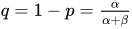
Values for the skewness and excess kurtosis below the lower boundary (excess kurtosis + 2 − skewness2 = 0) cannot occur for any distribution, and hence Karl Pearson appropriately called the region below this boundary the "impossible region". The boundary for this "impossible region" is determined by (symmetric or skewed) bimodal U-shaped distributions for which the parameters α and β approach zero and hence all the probability density is concentrated at the ends: x = 0, 1 with practically nothing in between them. Since for α ≈ β ≈ 0 the probability density is concentrated at the two ends x = 0 and x = 1, this "impossible boundary" is determined by a Bernoulli distribution, where the two only possible outcomes occur with respective probabilities p and q = 1 − p. For cases approaching this limit boundary with symmetry α = β, skewness ≈ 0, excess kurtosis ≈ −2 (this is the lowest excess kurtosis possible for any distribution), and the probabilities are p ≈ q ≈ 1/2. For cases approaching this limit boundary with skewness, excess kurtosis ≈ −2 + skewness2, and the probability density is concentrated more at one end than the other end (with practically nothing in between), with probabilities at the left end x = 0 and at the right end x = 1.

Symmetry
All statements are conditional on α, β > 0:
- Probability density functionreflection symmetry
- Cumulative distribution functionreflection symmetry plus unitary translation
- Modereflection symmetry plus unitary translation
- Medianreflection symmetry plus unitary translation
- Meanreflection symmetry plus unitary translation
- Geometric means each is individually asymmetric, the following symmetry applies between the geometric mean based on X and the geometric mean based on its reflection 1−X
- Harmonic means each is individually asymmetric, the following symmetry applies between the harmonic mean based on X and the harmonic mean based on its reflection 1−X
- Variance symmetry
- Geometric variances each is individually asymmetric, the following symmetry applies between the log geometric variance based on X and the log geometric variance based on its reflection 1−X
- Geometric covariance symmetry
- Mean absolute deviation around the mean symmetry
- Skewnessskew-symmetry
- Excess kurtosis symmetry
- Characteristic function symmetry of Real part (with respect to the origin of variable "t") ;\alpha +\beta ;it)]={\text{Re}}[{}_{1}F_{1}(\alpha ;\alpha +\beta ;-it)]}
- Characteristic functionskew-symmetry of Imaginary part (with respect to the origin of variable "t") ;\alpha +\beta ;it)]=-{\text{Im}}[{}_{1}F_{1}(\alpha ;\alpha +\beta ;-it)]}
- Characteristic function symmetry of Absolute value (with respect to the origin of variable "t") ;\alpha +\beta ;it)]={\text{Abs}}[{}_{1}F_{1}(\alpha ;\alpha +\beta ;-it)]}
- Differential entropy symmetry
- Relative entropy (also called Kullback–Leibler divergence) symmetry
- Fisher information matrix symmetry








![{\displaystyle \operatorname {E} [|X-E[X]|](\mathrm {B} (\alpha ,\beta ))=\operatorname {E} [|X-E[X]|](\mathrm {B} (\beta ,\alpha ))}](https://wikimedia.org/api/rest_v1/media/math/render/svg/83468b7365d9095b07e04bfbb5c9cff50c64ea2d)


![{\displaystyle {\text{Re}}[{}_{1}F_{1}(\alpha ;\alpha +\beta ;it)]={\text{Re}}[{}_{1}F_{1}(\alpha ;\alpha +\beta ;-it)]}](https://wikimedia.org/api/rest_v1/media/math/render/svg/55bbddff6ec53eb39eccc603618459ba36e10ad2)
![{\displaystyle {\text{Im}}[{}_{1}F_{1}(\alpha ;\alpha +\beta ;it)]=-{\text{Im}}[{}_{1}F_{1}(\alpha ;\alpha +\beta ;-it)]}](https://wikimedia.org/api/rest_v1/media/math/render/svg/ebb682c9915a60ef8d982340de042127ab262a0f)
![{\displaystyle {\text{Abs}}[{}_{1}F_{1}(\alpha ;\alpha +\beta ;it)]={\text{Abs}}[{}_{1}F_{1}(\alpha ;\alpha +\beta ;-it)]}](https://wikimedia.org/api/rest_v1/media/math/render/svg/08c1c15ff4c63020b66d2404d439514d965946d0)



Geometry of the probability density function
Inflection points


For certain values of the shape parameters α and β, the probability density function has inflection points, at which the curvature changes sign. The position of these inflection points can be useful as a measure of the dispersion or spread of the distribution.
Defining the following quantity:
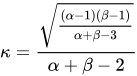
Points of inflection occur,[1][8][9][20] depending on the value of the shape parameters α and β, as follows:
- (α > 2, β > 2) The distribution is bell-shaped (symmetric for α = β and skewed otherwise), with two inflection points, equidistant from the mode:
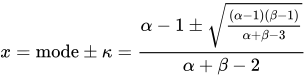
- (α = 2, β > 2) The distribution is unimodal, positively skewed, right-tailed, with one inflection point, located to the right of the mode:
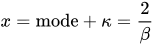
- (α > 2, β = 2) The distribution is unimodal, negatively skewed, left-tailed, with one inflection point, located to the left of the mode:
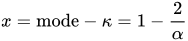
- (1 < α < 2, β > 2, α + β > 2) The distribution is unimodal, positively skewed, right-tailed, with one inflection point, located to the right of the mode:
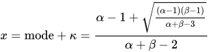
- (0 < α < 1, 1 < β < 2) The distribution has a mode at the left end x = 0 and it is positively skewed, right-tailed. There is one inflection point, located to the right of the mode:
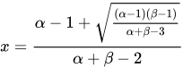
- (α > 2, 1 < β < 2) The distribution is unimodal negatively skewed, left-tailed, with one inflection point, located to the left of the mode:

- (1 < α < 2, 0 < β < 1) The distribution has a mode at the right end x = 1 and it is negatively skewed, left-tailed. There is one inflection point, located to the left of the mode:
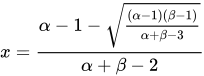
There are no inflection points in the remaining (symmetric and skewed) regions: U-shaped: (α, β < 1) upside-down-U-shaped: (1 < α < 2, 1 < β < 2), reverse-J-shaped (α < 1, β > 2) or J-shaped: (α > 2, β < 1)
The accompanying plots show the inflection point locations (shown vertically, ranging from 0 to 1) versus α and β (the horizontal axes ranging from 0 to 5). There are large cuts at surfaces intersecting the lines α = 1, β = 1, α = 2, and β = 2 because at these values the beta distribution change from 2 modes, to 1 mode to no mode.
Shapes


The beta density function can take a wide variety of different shapes depending on the values of the two parameters α and β. The ability of the beta distribution to take this great diversity of shapes (using only two parameters) is partly responsible for finding wide application for modeling actual measurements:
Symmetric (α = β)
- the density function is symmetric about 1/2 (blue & teal plots).
- median = mean = 1/2.
- skewness = 0.
- variance = 1/(4(2α + 1))
- α = β < 1
- U-shaped (blue plot).
- bimodal: left mode = 0, right mode =1, anti-mode = 1/2
- 1/12 < var(X) < 1/4[1]
- −2 < excess kurtosis(X) < −6/5
- α = β = 1/2 is the arcsine distribution
- var(X) = 1/8
- excess kurtosis(X) = −3/2
- CF = Rinc (t) [34]
- α = β → 0 is a 2-point Bernoulli distribution with equal probability 1/2 at each Dirac delta function end x = 0 and x = 1 and zero probability everywhere else. A coin toss: one face of the coin being x = 0 and the other face being x = 1.
- a lower value than this is impossible for any distribution to reach.
- The differential entropy approaches a minimum value of −∞
- α = β = 1
- the uniform [0, 1] distribution
- no mode
- var(X) = 1/12
- excess kurtosis(X) = −6/5
- The (negative anywhere else) differential entropy reaches its maximum value of zero
- CF = Sinc (t)
- α = β > 1
- symmetric unimodal
- mode = 1/2.
- 0 < var(X) < 1/12[1]
- −6/5 < excess kurtosis(X) < 0
- α = β = 3/2 is a semi-elliptic [0, 1] distribution, see: Wigner semicircle distribution[35]
- var(X) = 1/16.
- excess kurtosis(X) = −1
- CF = 2 Jinc (t)
- α = β = 2 is the parabolic [0, 1] distribution
- var(X) = 1/20
- excess kurtosis(X) = −6/7
- CF = 3 Tinc (t) [36]
- α = β > 2 is bell-shaped, with inflection points located to either side of the mode
- 0 < var(X) < 1/20
- −6/7 < excess kurtosis(X) < 0
- α = β → ∞ is a 1-point Degenerate distribution with a Dirac delta function spike at the midpoint x = 1/2 with probability 1, and zero probability everywhere else. There is 100% probability (absolute certainty) concentrated at the single point x = 1/2.
- The differential entropy approaches a minimum value of −∞
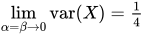

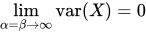

Skewed (α ≠ β)
The density function is skewed. An interchange of parameter values yields the mirror image (the reverse) of the initial curve, some more specific cases:
- α < 1, β < 1
- U-shaped
- Positive skew for α < β, negative skew for α > β.
- bimodal: left mode = 0, right mode = 1, anti-mode =
- 0 < median < 1.
- 0 < var(X) < 1/4
- α > 1, β > 1
- unimodal (magenta & cyan plots),
- Positive skew for α < β, negative skew for α > β.
- 0 < median < 1
- 0 < var(X) < 1/12
- α < 1, β ≥ 1
- reverse J-shaped with a right tail,
- positively skewed,
- strictly decreasing, convex
- mode = 0
- 0 < median < 1/2.
- (maximum variance occurs for , or α = Φ the golden ratio conjugate)
- α ≥ 1, β < 1
- J-shaped with a left tail,
- negatively skewed,
- strictly increasing, convex
- mode = 1
- 1/2 < median < 1
- (maximum variance occurs for , or β = Φ the golden ratio conjugate)
- α = 1, β > 1
- positively skewed,
- strictly decreasing (red plot),
- a reversed (mirror-image) power function distribution
- mean = 1 / (β + 1)
- median = 1 - 1/21/β
- mode = 0
- α = 1, 1 < β < 2
- concave
- 1/18 < var(X) < 1/12.
- α = 1, β = 2
- a straight line with slope −2, the right-triangular distribution with right angle at the left end, at x = 0
- var(X) = 1/18
- α = 1, β > 2
- reverse J-shaped with a right tail,
- convex
- 0 < var(X) < 1/18
- α > 1, β = 1
- negatively skewed,
- strictly increasing (green plot),
- the power function distribution[9]
- mean = α / (α + 1)
- median = 1/21/α
- mode = 1
- 2 > α > 1, β = 1
- concave
- 1/18 < var(X) < 1/12
- α = 2, β = 1
- a straight line with slope +2, the right-triangular distribution with right angle at the right end, at x = 1
- var(X) = 1/18
- α > 2, β = 1
- J-shaped with a left tail, convex
- 0 < var(X) < 1/18



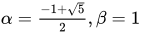
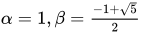

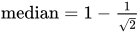

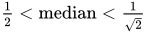
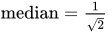
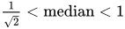
Related distributions
Transformations
- If X ~ Beta(α, β) then 1 − X ~ Beta(β, α) mirror-image symmetry
- If X ~ Beta(α, β) then . The beta prime distribution, also called "beta distribution of the second kind".
- If , then has a generalized logistic distribution, also called logistic-beta, with density , where is the logistic sigmoid.
- If X ~ Beta(α, β) then .
- If and then has density for and for , where is the Hypergeometric function.[37]
- If X ~ Beta(n/2, m/2) then (assuming n > 0 and m > 0), the Fisher–Snedecor F distribution.
- If then min + X(max − min) ~ PERT(min, max, m, λ) where PERT denotes a PERT distribution used in PERT analysis, and m=most likely value.[38] Traditionally[39]λ = 4 in PERT analysis.
- If X ~ Beta(1, β) then X ~ Kumaraswamy distribution with parameters (1, β)
- If X ~ Beta(α, 1) then X ~ Kumaraswamy distribution with parameters (α, 1)
- If X ~ Beta(α, 1) then −ln(X) ~ Exponential(α)


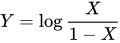
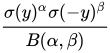

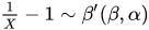


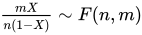

Special and limiting cases


- Beta(1, 1) ~ U(0, 1) with density 1 on that interval.
- Beta(n, 1) ~ Maximum of n independent rvs. with U(0, 1), sometimes called a a standard power function distribution with density n xn–1 on that interval.
- Beta(1, n) ~ Minimum of n independent rvs. with U(0, 1) with density n(1 − x)n−1 on that interval.
- If X ~ Beta(3/2, 3/2) and r > 0 then 2rX − r ~ Wigner semicircle distribution.
- Beta(1/2, 1/2) is equivalent to the arcsine distribution. This distribution is also Jeffreys prior probability for the Bernoulli and binomial distributions.
- the exponential distribution.
- the gamma distribution.
- For large , the normal distribution. More precisely, if then converges in distribution to a normal distribution with mean 0 and variance as n increases.





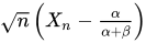

Derived from other distributions
- The kth order statistic of a sample of size n from the uniform distribution is a beta random variable, U(k) ~ Beta(k, n+1−k).[40]
- Gamma distribution: If X ~ Gamma(α, θ) and Y ~ Gamma(β, θ) are independent, then .
- Chi-squared distribution: If and are independent, then .
- The power transformation for the uniform distribution: If X ~ U(0, 1) and α > 0 then X1/α ~ Beta(α, 1).
- Cauchy distribution: If X ~ Cauchy(0, 1) then



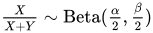
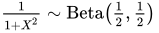
Combination with other distributions
- X ~ Beta(α, β) and Y ~ F(2β,2α) then for all x > 0.

Compounding with other distributions
- If p ~ Beta(α, β) and X ~ Bin(k, p) then X ~ beta-binomial distribution
- If p ~ Beta(α, β) and X ~ NB(r, p) then X ~ beta negative binomial distribution
Generalisations
- The multivariate generalization with sum-to-1 constraint is called a Dirichlet distribution. Univariate marginals of the Dirichlet distribution have a beta distribution. The beta distribution is conjugate to the binomial and Bernoulli distributions in exactly the same way as the Dirichlet distribution is conjugate to the multinomial distribution and categorical distribution.
- The multivariate Logistic-beta distribution[41] along with coordinate-wise logistic transformation can be considered as a multivariate generalization of beta distribution without sum-to-1 constraint. It is supported on the unit hypercube with common Beta(α, β) univariate marginals.
- The Pearson type I distribution is identical to the beta distribution (except for arbitrary shifting and re-scaling that can also be accomplished with the four parameter parametrization of the beta distribution).
- The beta distribution is the special case of the noncentral beta distribution where : .
- The generalized beta distribution is a five-parameter distribution family which has the beta distribution as a special case.
- The matrix variate beta distribution is a distribution for positive-definite matrices.


Statistical inference
Parameter estimation
Method of moments
Two unknown parameters
Two unknown parameters ( of a beta distribution supported in the [0,1] interval) can be estimated, using the method of moments, with the first two moments (sample mean and sample variance) as follows. Let:

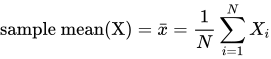
be the sample mean estimate and

be the sample variance estimate. The method-of-moments estimates of the parameters are


When the distribution is required over a known interval other than [0, 1] with random variable X, say [a, c] with random variable Y, then replace with and with in the above couple of equations for the shape parameters (see the "Four unknown parameters" section below),[42] where:


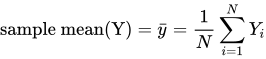

Four unknown parameters
All four parameters ( of a beta distribution supported in the [a, c] interval, see section "Alternative parametrizations, Four parameters") can be estimated, using the method of moments developed by Karl Pearson, by equating sample and population values of the first four central moments (mean, variance, skewness and excess kurtosis).[1][43][44] The excess kurtosis was expressed in terms of the square of the skewness, and the sample size ν = α + β, (see previous section "Kurtosis") as follows:


One can use this equation to solve for the sample size ν= α + β in terms of the square of the skewness and the excess kurtosis as follows:[43]


This is the ratio (multiplied by a factor of 3) between the previously derived limit boundaries for the beta distribution in a space (as originally done by Karl Pearson[21]) defined with coordinates of the square of the skewness in one axis and the excess kurtosis in the other axis (see § Kurtosis bounded by the square of the skewness):
The case of zero skewness, can be immediately solved because for zero skewness, α = β and hence ν = 2α = 2β, therefore α = β = ν/2


(Excess kurtosis is negative for the beta distribution with zero skewness, ranging from -2 to 0, so that -and therefore the sample shape parameters- is positive, ranging from zero when the shape parameters approach zero and the excess kurtosis approaches -2, to infinity when the shape parameters approach infinity and the excess kurtosis approaches zero).

For non-zero sample skewness one needs to solve a system of two coupled equations. Since the skewness and the excess kurtosis are independent of the parameters , the parameters can be uniquely determined from the sample skewness and the sample excess kurtosis, by solving the coupled equations with two known variables (sample skewness and sample excess kurtosis) and two unknowns (the shape parameters):


resulting in the following solution:[43]
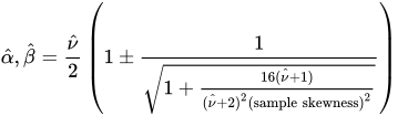

Where one should take the solutions as follows: for (negative) sample skewness < 0, and for (positive) sample skewness > 0.


The accompanying plot shows these two solutions as surfaces in a space with horizontal axes of (sample excess kurtosis) and (sample squared skewness) and the shape parameters as the vertical axis. The surfaces are constrained by the condition that the sample excess kurtosis must be bounded by the sample squared skewness as stipulated in the above equation. The two surfaces meet at the right edge defined by zero skewness. Along this right edge, both parameters are equal and the distribution is symmetric U-shaped for α = β < 1, uniform for α = β = 1, upside-down-U-shaped for 1 < α = β < 2 and bell-shaped for α = β > 2. The surfaces also meet at the front (lower) edge defined by "the impossible boundary" line (excess kurtosis + 2 - skewness2 = 0). Along this front (lower) boundary both shape parameters approach zero, and the probability density is concentrated more at one end than the other end (with practically nothing in between), with probabilities at the left end x = 0 and at the right end x = 1. The two surfaces become further apart towards the rear edge. At this rear edge the surface parameters are quite different from each other. As remarked, for example, by Bowman and Shenton,[45] sampling in the neighborhood of the line (sample excess kurtosis - (3/2)(sample skewness)2 = 0) (the just-J-shaped portion of the rear edge where blue meets beige), "is dangerously near to chaos", because at that line the denominator of the expression above for the estimate ν = α + β becomes zero and hence ν approaches infinity as that line is approached. Bowman and Shenton [45] write that "the higher moment parameters (kurtosis and skewness) are extremely fragile (near that line). However, the mean and standard deviation are fairly reliable." Therefore, the problem is for the case of four parameter estimation for very skewed distributions such that the excess kurtosis approaches (3/2) times the square of the skewness. This boundary line is produced by extremely skewed distributions with very large values of one of the parameters and very small values of the other parameter. See § Kurtosis bounded by the square of the skewness for a numerical example and further comments about this rear edge boundary line (sample excess kurtosis - (3/2)(sample skewness)2 = 0). As remarked by Karl Pearson himself [46] this issue may not be of much practical importance as this trouble arises only for very skewed J-shaped (or mirror-image J-shaped) distributions with very different values of shape parameters that are unlikely to occur much in practice). The usual skewed-bell-shape distributions that occur in practice do not have this parameter estimation problem.
The remaining two parameters can be determined using the sample mean and the sample variance using a variety of equations.[1][43] One alternative is to calculate the support interval range based on the sample variance and the sample kurtosis. For this purpose one can solve, in terms of the range , the equation expressing the excess kurtosis in terms of the sample variance, and the sample size ν (see § Kurtosis and § Alternative parametrizations, four parameters):


to obtain:

Another alternative is to calculate the support interval range based on the sample variance and the sample skewness.[43] For this purpose one can solve, in terms of the range , the equation expressing the squared skewness in terms of the sample variance, and the sample size ν (see section titled "Skewness" and "Alternative parametrizations, four parameters"):

to obtain:[43]

The remaining parameter can be determined from the sample mean and the previously obtained parameters: :


and finally, .

In the above formulas one may take, for example, as estimates of the sample moments:
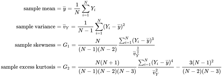
The estimators G1 for sample skewness and G2 for sample kurtosis are used by DAP/SAS, PSPP/SPSS, and Excel. However, they are not used by BMDP and (according to [47]) they were not used by MINITAB in 1998. Actually, Joanes and Gill in their 1998 study[47] concluded that the skewness and kurtosis estimators used in BMDP and in MINITAB (at that time) had smaller variance and mean-squared error in normal samples, but the skewness and kurtosis estimators used in DAP/SAS, PSPP/SPSS, namely G1 and G2, had smaller mean-squared error in samples from a very skewed distribution. It is for this reason that we have spelled out "sample skewness", etc., in the above formulas, to make it explicit that the user should choose the best estimator according to the problem at hand, as the best estimator for skewness and kurtosis depends on the amount of skewness (as shown by Joanes and Gill[47]).
Maximum likelihood
Two unknown parameters


As is also the case for maximum likelihood estimates for the gamma distribution, the maximum likelihood estimates for the beta distribution do not have a general closed form solution for arbitrary values of the shape parameters. If X1, ..., XN are independent random variables each having a beta distribution, the joint log likelihood function for Niid observations is:

Finding the maximum with respect to a shape parameter involves taking the partial derivative with respect to the shape parameter and setting the expression equal to zero yielding the maximum likelihood estimator of the shape parameters:


where:
![{\displaystyle {\begin{aligned}{\frac {\partial \ln \mathrm {B} (\alpha ,\beta )}{\partial \alpha }}&=-{\frac {\partial \ln \Gamma (\alpha +\beta )}{\partial \alpha }}+{\frac {\partial \ln \Gamma (\alpha )}{\partial \alpha }}+{\frac {\partial \ln \Gamma (\beta )}{\partial \alpha }}\\[1ex]&=-\psi (\alpha +\beta )+\psi (\alpha )+0\end{aligned}}}](https://wikimedia.org/api/rest_v1/media/math/render/svg/82bf10edac73617ec99a3adbad3ff020391c4a71)
![{\displaystyle {\begin{aligned}{\frac {\partial \ln \mathrm {B} (\alpha ,\beta )}{\partial \beta }}&=-{\frac {\partial \ln \Gamma (\alpha +\beta )}{\partial \beta }}+{\frac {\partial \ln \Gamma (\alpha )}{\partial \beta }}+{\frac {\partial \ln \Gamma (\beta )}{\partial \beta }}\\[1ex]&=-\psi (\alpha +\beta )+0+\psi (\beta )\end{aligned}}}](https://wikimedia.org/api/rest_v1/media/math/render/svg/10b097547a81011b4e212824977d66b5350dc780)
since the digamma function denoted ψ(α) is defined as the logarithmic derivative of the gamma function:[18]
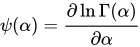
To ensure that the values with zero tangent slope are indeed a maximum (instead of a saddle-point or a minimum) one has to also satisfy the condition that the curvature is negative. This amounts to satisfying that the second partial derivative with respect to the shape parameters is negative


using the previous equations, this is equivalent to:


where the trigamma function, denoted ψ1(α), is the second of the polygamma functions, and is defined as the derivative of the digamma function:

These conditions are equivalent to stating that the variances of the logarithmically transformed variables are positive, since:
![{\displaystyle \operatorname {var} [\ln(X)]=\operatorname {E} [\ln ^{2}(X)]-(\operatorname {E} [\ln(X)])^{2}=\psi _{1}(\alpha )-\psi _{1}(\alpha +\beta )}](https://wikimedia.org/api/rest_v1/media/math/render/svg/d7737d681fea7490e27f8760c6bcc8fccb154904)
![{\displaystyle \operatorname {var} [\ln(1-X)]=\operatorname {E} [\ln ^{2}(1-X)]-(\operatorname {E} [\ln(1-X)])^{2}=\psi _{1}(\beta )-\psi _{1}(\alpha +\beta )}](https://wikimedia.org/api/rest_v1/media/math/render/svg/f84c3747955206cf2190c61bd7875a6cd739ac04)
Therefore, the condition of negative curvature at a maximum is equivalent to the statements:
![{\displaystyle \operatorname {var} [\ln(X)]>0}](https://wikimedia.org/api/rest_v1/media/math/render/svg/5fb5a5d0db057469fb9dad8df2902fe93e3f3b0d)
![{\displaystyle \operatorname {var} [\ln(1-X)]>0}](https://wikimedia.org/api/rest_v1/media/math/render/svg/c66a5aaa8362f578beb9b141b4108138b9d21e89)
Alternatively, the condition of negative curvature at a maximum is also equivalent to stating that the following logarithmic derivatives of the geometric meansGX and G(1−X) are positive, since:


While these slopes are indeed positive, the other slopes are negative:

The slopes of the mean and the median with respect to α and β display similar sign behavior.
From the condition that at a maximum, the partial derivative with respect to the shape parameter equals zero, we obtain the following system of coupled maximum likelihood estimate equations (for the average log-likelihoods) that needs to be inverted to obtain the (unknown) shape parameter estimates in terms of the (known) average of logarithms of the samples X1, ..., XN:[1]
![{\displaystyle {\begin{aligned}{\hat {\operatorname {E} }}[\ln(X)]&=\psi ({\hat {\alpha }})-\psi ({\hat {\alpha }}+{\hat {\beta }})={\frac {1}{N}}\sum _{i=1}^{N}\ln X_{i}=\ln {\hat {G}}_{X}\\{\hat {\operatorname {E} }}[\ln(1-X)]&=\psi ({\hat {\beta }})-\psi ({\hat {\alpha }}+{\hat {\beta }})={\frac {1}{N}}\sum _{i=1}^{N}\ln(1-X_{i})=\ln {\hat {G}}_{1-X}\end{aligned}}}](https://wikimedia.org/api/rest_v1/media/math/render/svg/42f099a4869ce2d200dc80c7675a237caae021e6)
where we recognize as the logarithm of the sample geometric mean and as the logarithm of the sample geometric mean based on (1 − X), the mirror-image of X. For , it follows that .


These coupled equations containing digamma functions of the shape parameter estimates must be solved by numerical methods as done, for example, by Beckman et al.[48] Gnanadesikan et al. give numerical solutions for a few cases.[49]N.L.Johnson and S.Kotz[1] suggest that for "not too small" shape parameter estimates , the logarithmic approximation to the digamma function may be used to obtain initial values for an iterative solution, since the equations resulting from this approximation can be solved exactly:

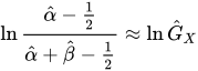

which leads to the following solution for the initial values (of the estimate shape parameters in terms of the sample geometric means) for an iterative solution:


Alternatively, the estimates provided by the method of moments can instead be used as initial values for an iterative solution of the maximum likelihood coupled equations in terms of the digamma functions.
When the distribution is required over a known interval other than [0, 1] with random variable X, say [a, c] with random variable Y, then replace ln(Xi) in the first equation with

and replace ln(1−Xi) in the second equation with

(see "Alternative parametrizations, four parameters" section below).
If one of the shape parameters is known, the problem is considerably simplified. The following logit transformation can be used to solve for the unknown shape parameter (for skewed cases such that , otherwise, if symmetric, both -equal- parameters are known when one is known):

![{\displaystyle {\hat {\operatorname {E} }}\left[\ln {\frac {X}{1-X}}\right]=\psi ({\hat {\alpha }})-\psi ({\hat {\beta }})={\frac {1}{N}}\sum _{i=1}^{N}\ln {\frac {X_{i}}{1-X_{i}}}=\ln {\hat {G}}_{X}-\ln {\hat {G}}_{1-X}}](https://wikimedia.org/api/rest_v1/media/math/render/svg/ca41c85f9e8cd1b427e96fd209fea0522c951d65)
This logit transformation is the logarithm of the transformation that divides the variable X by its mirror-image (X/(1 - X) resulting in the "inverted beta distribution" or beta prime distribution (also known as beta distribution of the second kind or Pearson's Type VI) with support [0, +∞). As previously discussed in the section "Moments of logarithmically transformed random variables," the logit transformation , studied by Johnson,[25] extends the finite support [0, 1] based on the original variable X to infinite support in both directions of the real line (−∞, +∞).

If, for example, is known, the unknown parameter can be obtained in terms of the inverse[50] digamma function of the right hand side of this equation:


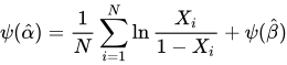

In particular, if one of the shape parameters has a value of unity, for example for (the power function distribution with bounded support [0,1]), using the identity ψ(x + 1) = ψ(x) + 1/x in the equation , the maximum likelihood estimator for the unknown parameter is,[1] exactly:


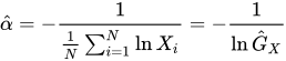
The beta has support [0, 1], therefore , and hence , and therefore

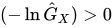

In conclusion, the maximum likelihood estimates of the shape parameters of a beta distribution are (in general) a complicated function of the sample geometric mean, and of the sample geometric mean based on (1−X)), the mirror-image of X. One may ask, if the variance (in addition to the mean) is necessary to estimate two shape parameters with the method of moments, why is the (logarithmic or geometric) variance not necessary to estimate two shape parameters with the maximum likelihood method, for which only the geometric means suffice? The answer is because the mean does not provide as much information as the geometric mean. For a beta distribution with equal shape parameters α = β, the mean is exactly 1/2, regardless of the value of the shape parameters, and therefore regardless of the value of the statistical dispersion (the variance). On the other hand, the geometric mean of a beta distribution with equal shape parameters α = β, depends on the value of the shape parameters, and therefore it contains more information. Also, the geometric mean of a beta distribution does not satisfy the symmetry conditions satisfied by the mean, therefore, by employing both the geometric mean based on X and geometric mean based on (1 − X), the maximum likelihood method is able to provide best estimates for both parameters α = β, without need of employing the variance.
One can express the joint log likelihood per Niid observations in terms of the sufficient statistics (the sample geometric means) as follows:

We can plot the joint log likelihood per N observations for fixed values of the sample geometric means to see the behavior of the likelihood function as a function of the shape parameters α and β. In such a plot, the shape parameter estimators correspond to the maxima of the likelihood function. See the accompanying graph that shows that all the likelihood functions intersect at α = β = 1, which corresponds to the values of the shape parameters that give the maximum entropy (the maximum entropy occurs for shape parameters equal to unity: the uniform distribution). It is evident from the plot that the likelihood function gives sharp peaks for values of the shape parameter estimators close to zero, but that for values of the shape parameters estimators greater than one, the likelihood function becomes quite flat, with less defined peaks. Obviously, the maximum likelihood parameter estimation method for the beta distribution becomes less acceptable for larger values of the shape parameter estimators, as the uncertainty in the peak definition increases with the value of the shape parameter estimators. One can arrive at the same conclusion by noticing that the expression for the curvature of the likelihood function is in terms of the geometric variances
![{\displaystyle {\frac {\partial ^{2}\ln {\mathcal {L}}(\alpha ,\beta \mid X)}{\partial \alpha ^{2}}}=-\operatorname {var} [\ln X]}](https://wikimedia.org/api/rest_v1/media/math/render/svg/517a09a3b13d22689a3e1e400cbcab3af08e130c)
![{\displaystyle {\frac {\partial ^{2}\ln {\mathcal {L}}(\alpha ,\beta \mid X)}{\partial \beta ^{2}}}=-\operatorname {var} [\ln(1-X)]}](https://wikimedia.org/api/rest_v1/media/math/render/svg/1715f50fc408ceba307005a3f9e404520edd5a20)
These variances (and therefore the curvatures) are much larger for small values of the shape parameter α and β. However, for shape parameter values α, β > 1, the variances (and therefore the curvatures) flatten out. Equivalently, this result follows from the Cramér–Rao bound, since the Fisher information matrix components for the beta distribution are these logarithmic variances. The Cramér–Rao bound states that the variance of any unbiased estimator of α is bounded by the reciprocal of the Fisher information:
![{\displaystyle \mathrm {var} ({\hat {\alpha }})\geq {\frac {1}{\operatorname {var} [\ln X]}}\geq {\frac {1}{\psi _{1}({\hat {\alpha }})-\psi _{1}({\hat {\alpha }}+{\hat {\beta }})}}}](https://wikimedia.org/api/rest_v1/media/math/render/svg/744f1e8421337ed7a2e6cae00fccec1eaf68e3dc)
![{\displaystyle \mathrm {var} ({\hat {\beta }})\geq {\frac {1}{\operatorname {var} [\ln(1-X)]}}\geq {\frac {1}{\psi _{1}({\hat {\beta }})-\psi _{1}({\hat {\alpha }}+{\hat {\beta }})}}}](https://wikimedia.org/api/rest_v1/media/math/render/svg/f01dc5c3eb614cfa71a500fd34f3fa430c183c76)
so the variance of the estimators increases with increasing α and β, as the logarithmic variances decrease.
Also one can express the joint log likelihood per Niid observations in terms of the digamma function expressions for the logarithms of the sample geometric means as follows:

this expression is identical to the negative of the cross-entropy (see section on "Quantities of information (entropy)"). Therefore, finding the maximum of the joint log likelihood of the shape parameters, per Niid observations, is identical to finding the minimum of the cross-entropy for the beta distribution, as a function of the shape parameters.

with the cross-entropy defined as follows:

Four unknown parameters
The procedure is similar to the one followed in the two unknown parameter case. If Y1, ..., YN are independent random variables each having a beta distribution with four parameters, the joint log likelihood function for Niid observations is:

Finding the maximum with respect to a shape parameter involves taking the partial derivative with respect to the shape parameter and setting the expression equal to zero yielding the maximum likelihood estimator of the shape parameters:




these equations can be re-arranged as the following system of four coupled equations (the first two equations are geometric means and the second two equations are the harmonic means) in terms of the maximum likelihood estimates for the four parameters :


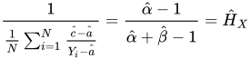
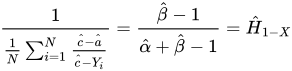
with sample geometric means:
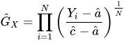
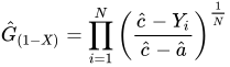
The parameters are embedded inside the geometric mean expressions in a nonlinear way (to the power 1/N). This precludes, in general, a closed form solution, even for an initial value approximation for iteration purposes. One alternative is to use as initial values for iteration the values obtained from the method of moments solution for the four parameter case. Furthermore, the expressions for the harmonic means are well-defined only for , which precludes a maximum likelihood solution for shape parameters less than unity in the four-parameter case. Fisher's information matrix for the four parameter case is positive-definite only for α, β > 2 (for further discussion, see section on Fisher information matrix, four parameter case), for bell-shaped (symmetric or unsymmetric) beta distributions, with inflection points located to either side of the mode. The following Fisher information components (that represent the expectations of the curvature of the log likelihood function) have singularities at the following values:

![{\displaystyle \alpha =2:\quad \operatorname {E} \left[-{\frac {1}{N}}{\frac {\partial ^{2}\ln {\mathcal {L}}(\alpha ,\beta ,a,c\mid Y)}{\partial a^{2}}}\right]={\mathcal {I}}_{a,a}}](https://wikimedia.org/api/rest_v1/media/math/render/svg/53538160a2404a5d7b74ae2033fbbb2dbc1045eb)
![{\displaystyle \beta =2:\quad \operatorname {E} \left[-{\frac {1}{N}}{\frac {\partial ^{2}\ln {\mathcal {L}}(\alpha ,\beta ,a,c\mid Y)}{\partial c^{2}}}\right]={\mathcal {I}}_{c,c}}](https://wikimedia.org/api/rest_v1/media/math/render/svg/ee2c6ecfcafe60e54799ab4a16451cf478d65f7d)
![{\displaystyle \alpha =2:\quad \operatorname {E} \left[-{\frac {1}{N}}{\frac {\partial ^{2}\ln {\mathcal {L}}(\alpha ,\beta ,a,c\mid Y)}{\partial \alpha \partial a}}\right]={\mathcal {I}}_{\alpha ,a}}](https://wikimedia.org/api/rest_v1/media/math/render/svg/8b8af544d7c5e0cc278aa725daba7f3de2f70d31)
![{\displaystyle \beta =1:\quad \operatorname {E} \left[-{\frac {1}{N}}{\frac {\partial ^{2}\ln {\mathcal {L}}(\alpha ,\beta ,a,c\mid Y)}{\partial \beta \partial c}}\right]={\mathcal {I}}_{\beta ,c}}](https://wikimedia.org/api/rest_v1/media/math/render/svg/2f87b32b39997964dcbc95bc64c1364e6832db1d)
(for further discussion see section on Fisher information matrix). Thus, it is not possible to strictly carry on the maximum likelihood estimation for some well known distributions belonging to the four-parameter beta distribution family, like the uniform distribution (Beta(1, 1, a, c)), and the arcsine distribution (Beta(1/2, 1/2, a, c)). N.L.Johnson and S.Kotz[1] ignore the equations for the harmonic means and instead suggest "If a and c are unknown, and maximum likelihood estimators of a, c, α and β are required, the above procedure (for the two unknown parameter case, with X transformed as X = (Y − a)/(c − a)) can be repeated using a succession of trial values of a and c, until the pair (a, c) for which maximum likelihood (given a and c) is as great as possible, is attained" (where, for the purpose of clarity, their notation for the parameters has been translated into the present notation).
Fisher information matrix
Let a random variable X have a probability density f(x;α). The partial derivative with respect to the (unknown, and to be estimated) parameter α of the log likelihood function is called the score. The second moment of the score is called the Fisher information:
![{\displaystyle {\mathcal {I}}(\alpha )=\operatorname {E} \left[\left({\frac {\partial }{\partial \alpha }}\ln {\mathcal {L}}(\alpha \mid X)\right)^{2}\right],}](https://wikimedia.org/api/rest_v1/media/math/render/svg/daec13972d17a073bcd447abfde55a6b0e168720)
The expectation of the score is zero, therefore the Fisher information is also the second moment centered on the mean of the score: the variance of the score.
If the log likelihood function is twice differentiable with respect to the parameter α, and under certain regularity conditions,[51] then the Fisher information may also be written as follows (which is often a more convenient form for calculation purposes):
![{\displaystyle {\mathcal {I}}(\alpha )=-\operatorname {E} \left[{\frac {\partial ^{2}}{\partial \alpha ^{2}}}\ln {\mathcal {L}}(\alpha \mid X)\right].}](https://wikimedia.org/api/rest_v1/media/math/render/svg/3fdd5f6730d5ffb0a5f833c89ba784362322cbc8)
Thus, the Fisher information is the negative of the expectation of the second derivative with respect to the parameter α of the log likelihood function. Therefore, Fisher information is a measure of the curvature of the log likelihood function of α. A low curvature (and therefore high radius of curvature), flatter log likelihood function curve has low Fisher information; while a log likelihood function curve with large curvature (and therefore low radius of curvature) has high Fisher information. When the Fisher information matrix is computed at the evaluates of the parameters ("the observed Fisher information matrix") it is equivalent to the replacement of the true log likelihood surface by a Taylor's series approximation, taken as far as the quadratic terms.[52] The word information, in the context of Fisher information, refers to information about the parameters. Information such as: estimation, sufficiency and properties of variances of estimators. The Cramér–Rao bound states that the inverse of the Fisher information is a lower bound on the variance of any estimator of a parameter α:
![{\displaystyle \operatorname {var} [{\hat {\alpha }}]\geq {\frac {1}{{\mathcal {I}}(\alpha )}}.}](https://wikimedia.org/api/rest_v1/media/math/render/svg/d93d4983a2717258c52eb47d1562e849a3a66c5c)
The precision to which one can estimate the estimator of a parameter α is limited by the Fisher Information of the log likelihood function. The Fisher information is a measure of the minimum error involved in estimating a parameter of a distribution and it can be viewed as a measure of the resolving power of an experiment needed to discriminate between two alternative hypothesis of a parameter.[53]
When there are N parameters
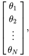
then the Fisher information takes the form of an N×Npositive semidefinitesymmetric matrix, the Fisher information matrix, with typical element:
![{\displaystyle ({\mathcal {I}}(\theta ))_{i,j}=\operatorname {E} \left[{\frac {\partial \ln {\mathcal {L}}}{\partial \theta _{i}}}\cdot {\frac {\partial \ln {\mathcal {L}}}{\partial \theta _{j}}}\right].}](https://wikimedia.org/api/rest_v1/media/math/render/svg/94187c0032daae02409e5323c356fae5fdcb73fd)
Under certain regularity conditions,[51] the Fisher Information Matrix may also be written in the following form, which is often more convenient for computation:
![{\displaystyle ({\mathcal {I}}(\theta ))_{i,j}=-\operatorname {E} \left[{\frac {\partial ^{2}\ln {\mathcal {L}}}{\partial \theta _{i}\,\partial \theta _{j}}}\right]\,.}](https://wikimedia.org/api/rest_v1/media/math/render/svg/86df084593df54dd2ed7220a683b9fbc41f230d7)
With X1, ..., XNiid random variables, an N-dimensional "box" can be constructed with sides X1, ..., XN. Costa and Cover[54] show that the (Shannon) differential entropy h(X) is related to the volume of the typical set (having the sample entropy close to the true entropy), while the Fisher information is related to the surface of this typical set.
Two parameters
For X1, ..., XN independent random variables each having a beta distribution parametrized with shape parameters α and β, the joint log likelihood function for Niid observations is:

therefore the joint log likelihood function per Niid observations is

For the two parameter case, the Fisher information has 4 components: 2 diagonal and 2 off-diagonal. Since the Fisher information matrix is symmetric, one of these off diagonal components is independent. Therefore, the Fisher information matrix has 3 independent components (2 diagonal and 1 off diagonal).
Aryal and Nadarajah[55] calculated Fisher's information matrix for the four-parameter case, from which the two parameter case can be obtained as follows:
![{\displaystyle -{\frac {\partial ^{2}\ln {\mathcal {L}}(\alpha ,\beta \mid X)}{N\partial \alpha ^{2}}}=\operatorname {var} [\ln(X)]=\psi _{1}(\alpha )-\psi _{1}(\alpha +\beta )={\mathcal {I}}_{\alpha ,\alpha }=\operatorname {E} \left[-{\frac {\partial ^{2}\ln {\mathcal {L}}(\alpha ,\beta \mid X)}{N\partial \alpha ^{2}}}\right]=\ln \operatorname {var} _{GX}}](https://wikimedia.org/api/rest_v1/media/math/render/svg/c90003d5bd2f6d2bcfe2c788585689726b4b7e36)
![{\displaystyle -{\frac {\partial ^{2}\ln {\mathcal {L}}(\alpha ,\beta \mid X)}{N\,\partial \beta ^{2}}}=\operatorname {var} [\ln(1-X)]=\psi _{1}(\beta )-\psi _{1}(\alpha +\beta )={\mathcal {I}}_{\beta ,\beta }=\operatorname {E} \left[-{\frac {\partial ^{2}\ln {\mathcal {L}}(\alpha ,\beta \mid X)}{N\partial \beta ^{2}}}\right]=\ln \operatorname {var} _{G(1-X)}}](https://wikimedia.org/api/rest_v1/media/math/render/svg/b59bcc31f14f1f4b3b07bd92a66426bb6ac126b1)
![{\displaystyle -{\frac {\partial ^{2}\ln {\mathcal {L}}(\alpha ,\beta \mid X)}{N\,\partial \alpha \,\partial \beta }}=\operatorname {cov} [\ln X,\ln(1-X)]=-\psi _{1}(\alpha +\beta )={\mathcal {I}}_{\alpha ,\beta }=\operatorname {E} \left[-{\frac {\partial ^{2}\ln {\mathcal {L}}(\alpha ,\beta \mid X)}{N\,\partial \alpha \,\partial \beta }}\right]=\ln \operatorname {cov} _{G{X,(1-X)}}}](https://wikimedia.org/api/rest_v1/media/math/render/svg/a6c3268da3b23c062ce981ab02d4c454a0267365)
Since the Fisher information matrix is symmetric

The Fisher information components are equal to the log geometric variances and log geometric covariance. Therefore, they can be expressed as trigamma functions, denoted ψ1(α), the second of the polygamma functions, defined as the derivative of the digamma function:
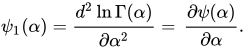
These derivatives are also derived in the § Two unknown parameters and plots of the log likelihood function are also shown in that section. § Geometric variance and covariance contains plots and further discussion of the Fisher information matrix components: the log geometric variances and log geometric covariance as a function of the shape parameters α and β. § Moments of logarithmically transformed random variables contains formulas for moments of logarithmically transformed random variables. Images for the Fisher information components and are shown in § Geometric variance.


The determinant of Fisher's information matrix is of interest (for example for the calculation of Jeffreys prior probability). From the expressions for the individual components of the Fisher information matrix, it follows that the determinant of Fisher's (symmetric) information matrix for the beta distribution is:
![{\displaystyle {\begin{aligned}\det({\mathcal {I}}(\alpha ,\beta ))&={\mathcal {I}}_{\alpha ,\alpha }{\mathcal {I}}_{\beta ,\beta }-{\mathcal {I}}_{\alpha ,\beta }{\mathcal {I}}_{\alpha ,\beta }\\[4pt]&=(\psi _{1}(\alpha )-\psi _{1}(\alpha +\beta ))(\psi _{1}(\beta )-\psi _{1}(\alpha +\beta ))-(-\psi _{1}(\alpha +\beta ))(-\psi _{1}(\alpha +\beta ))\\[4pt]&=\psi _{1}(\alpha )\psi _{1}(\beta )-(\psi _{1}(\alpha )+\psi _{1}(\beta ))\psi _{1}(\alpha +\beta )\\[4pt]\lim _{\alpha \to 0}\det({\mathcal {I}}(\alpha ,\beta ))&=\lim _{\beta \to 0}\det({\mathcal {I}}(\alpha ,\beta ))=\infty \\[4pt]\lim _{\alpha \to \infty }\det({\mathcal {I}}(\alpha ,\beta ))&=\lim _{\beta \to \infty }\det({\mathcal {I}}(\alpha ,\beta ))=0\end{aligned}}}](https://wikimedia.org/api/rest_v1/media/math/render/svg/b2c5ccf59b05ea730fc108360c07e9ac9634e829)
From Sylvester's criterion (checking whether the diagonal elements are all positive), it follows that the Fisher information matrix for the two parameter case is positive-definite (under the standard condition that the shape parameters are positive α > 0 and β > 0).
Four parameters


If Y1, ..., YN are independent random variables each having a beta distribution with four parameters: the exponents α and β, and also a (the minimum of the distribution range), and c (the maximum of the distribution range) (section titled "Alternative parametrizations", "Four parameters"), with probability density function:

the joint log likelihood function per Niid observations is:

For the four parameter case, the Fisher information has 4*4=16 components. It has 12 off-diagonal components = (4×4 total − 4 diagonal). Since the Fisher information matrix is symmetric, half of these components (12/2=6) are independent. Therefore, the Fisher information matrix has 6 independent off-diagonal + 4 diagonal = 10 independent components. Aryal and Nadarajah[55] calculated Fisher's information matrix for the four parameter case as follows:
![{\displaystyle -{\frac {1}{N}}{\frac {\partial ^{2}\ln {\mathcal {L}}(\alpha ,\beta ,a,c\mid Y)}{\partial \alpha ^{2}}}=\operatorname {var} [\ln(X)]=\psi _{1}(\alpha )-\psi _{1}(\alpha +\beta )={\mathcal {I}}_{\alpha ,\alpha }=\operatorname {E} \left[-{\frac {1}{N}}{\frac {\partial ^{2}\ln {\mathcal {L}}(\alpha ,\beta ,a,c\mid Y)}{\partial \alpha ^{2}}}\right]=\ln(\operatorname {var_{GX}} )}](https://wikimedia.org/api/rest_v1/media/math/render/svg/31be86f2c53663c6d3975bc2676806ba3e538423)
![{\displaystyle -{\frac {1}{N}}{\frac {\partial ^{2}\ln {\mathcal {L}}(\alpha ,\beta ,a,c\mid Y)}{\partial \beta ^{2}}}=\operatorname {var} [\ln(1-X)]=\psi _{1}(\beta )-\psi _{1}(\alpha +\beta )={\mathcal {I}}_{\beta ,\beta }=\operatorname {E} \left[-{\frac {1}{N}}{\frac {\partial ^{2}\ln {\mathcal {L}}(\alpha ,\beta ,a,c\mid Y)}{\partial \beta ^{2}}}\right]=\ln(\operatorname {var_{G(1-X)}} )}](https://wikimedia.org/api/rest_v1/media/math/render/svg/25ab885119f25fae0b9919326db96395d13e3bc3)
![{\displaystyle -{\frac {1}{N}}{\frac {\partial ^{2}\ln {\mathcal {L}}(\alpha ,\beta ,a,c\mid Y)}{\partial \alpha \,\partial \beta }}=\operatorname {cov} [\ln X,(1-X)]=-\psi _{1}(\alpha +\beta )={\mathcal {I}}_{\alpha ,\beta }=\operatorname {E} \left[-{\frac {1}{N}}{\frac {\partial ^{2}\ln {\mathcal {L}}(\alpha ,\beta ,a,c\mid Y)}{\partial \alpha \,\partial \beta }}\right]=\ln(\operatorname {cov} _{G{X,(1-X)}})}](https://wikimedia.org/api/rest_v1/media/math/render/svg/02a56af746fb9315340cf382951fe0c3f3640678)
In the above expressions, the use of X instead of Y in the expressions var[ln(X)] = ln(varGX) is not an error. The expressions in terms of the log geometric variances and log geometric covariance occur as functions of the two parameter X ~ Beta(α, β) parametrization because when taking the partial derivatives with respect to the exponents (α, β) in the four parameter case, one obtains the identical expressions as for the two parameter case: these terms of the four parameter Fisher information matrix are independent of the minimum a and maximum c of the distribution's range. The only non-zero term upon double differentiation of the log likelihood function with respect to the exponents α and β is the second derivative of the log of the beta function: ln(B(α, β)). This term is independent of the minimum a and maximum c of the distribution's range. Double differentiation of this term results in trigamma functions. The sections titled "Maximum likelihood", "Two unknown parameters" and "Four unknown parameters" also show this fact.
The Fisher information for Ni.i.d. samples is N times the individual Fisher information (eq. 11.279, page 394 of Cover and Thomas[28]). (Aryal and Nadarajah[55] take a single observation, N = 1, to calculate the following components of the Fisher information, which leads to the same result as considering the derivatives of the log likelihood per N observations. Moreover, below the erroneous expression for in Aryal and Nadarajah has been corrected.)

![{\displaystyle {\begin{aligned}\alpha >2:\quad \operatorname {E} \left[-{\frac {1}{N}}{\frac {\partial ^{2}\ln {\mathcal {L}}(\alpha ,\beta ,a,c\mid Y)}{\partial a^{2}}}\right]&={\mathcal {I}}_{a,a}={\frac {\beta (\alpha +\beta -1)}{(\alpha -2)(c-a)^{2}}}\\\beta >2:\quad \operatorname {E} \left[-{\frac {1}{N}}{\frac {\partial ^{2}\ln {\mathcal {L}}(\alpha ,\beta ,a,c\mid Y)}{\partial c^{2}}}\right]&={\mathcal {I}}_{c,c}={\frac {\alpha (\alpha +\beta -1)}{(\beta -2)(c-a)^{2}}}\\\operatorname {E} \left[-{\frac {1}{N}}{\frac {\partial ^{2}\ln {\mathcal {L}}(\alpha ,\beta ,a,c\mid Y)}{\partial a\,\partial c}}\right]&={\mathcal {I}}_{a,c}={\frac {(\alpha +\beta -1)}{(c-a)^{2}}}\\\alpha >1:\quad \operatorname {E} \left[-{\frac {1}{N}}{\frac {\partial ^{2}\ln {\mathcal {L}}(\alpha ,\beta ,a,c\mid Y)}{\partial \alpha \,\partial a}}\right]&={\mathcal {I}}_{\alpha ,a}={\frac {\beta }{(\alpha -1)(c-a)}}\\\operatorname {E} \left[-{\frac {1}{N}}{\frac {\partial ^{2}\ln {\mathcal {L}}(\alpha ,\beta ,a,c\mid Y)}{\partial \alpha \,\partial c}}\right]&={\mathcal {I}}_{\alpha ,c}={\frac {1}{(c-a)}}\\\operatorname {E} \left[-{\frac {1}{N}}{\frac {\partial ^{2}\ln {\mathcal {L}}(\alpha ,\beta ,a,c\mid Y)}{\partial \beta \,\partial a}}\right]&={\mathcal {I}}_{\beta ,a}=-{\frac {1}{(c-a)}}\\\beta >1:\quad \operatorname {E} \left[-{\frac {1}{N}}{\frac {\partial ^{2}\ln {\mathcal {L}}(\alpha ,\beta ,a,c\mid Y)}{\partial \beta \,\partial c}}\right]&={\mathcal {I}}_{\beta ,c}=-{\frac {\alpha }{(\beta -1)(c-a)}}\end{aligned}}}](https://wikimedia.org/api/rest_v1/media/math/render/svg/636646f51bdb1a3193b1721483878e98f4f19c3e)
The lower two diagonal entries of the Fisher information matrix, with respect to the parameter a (the minimum of the distribution's range): , and with respect to the parameter c (the maximum of the distribution's range): are only defined for exponents α > 2 and β > 2 respectively. The Fisher information matrix component for the minimum a approaches infinity for exponent α approaching 2 from above, and the Fisher information matrix component for the maximum c approaches infinity for exponent β approaching 2 from above.

The Fisher information matrix for the four parameter case does not depend on the individual values of the minimum a and the maximum c, but only on the total range (c − a). Moreover, the components of the Fisher information matrix that depend on the range (c − a), depend only through its inverse (or the square of the inverse), such that the Fisher information decreases for increasing range (c − a).
The accompanying images show the Fisher information components and . Images for the Fisher information components and are shown in § Geometric variance. All these Fisher information components look like a basin, with the "walls" of the basin being located at low values of the parameters.


The following four-parameter-beta-distribution Fisher information components can be expressed in terms of the two-parameter: X ~ Beta(α, β) expectations of the transformed ratio ((1 − X)/X) and of its mirror image (X/(1 − X)), scaled by the range (c − a), which may be helpful for interpretation:
![{\displaystyle {\mathcal {I}}_{\alpha ,a}={\frac {\operatorname {E} \left[{\frac {1-X}{X}}\right]}{c-a}}={\frac {\beta }{(\alpha -1)(c-a)}}{\text{ if }}\alpha >1}](https://wikimedia.org/api/rest_v1/media/math/render/svg/e670565bb8d06bace69cf892864520f5c83b5449)
![{\displaystyle {\mathcal {I}}_{\beta ,c}=-{\frac {\operatorname {E} \left[{\frac {X}{1-X}}\right]}{c-a}}=-{\frac {\alpha }{(\beta -1)(c-a)}}{\text{ if }}\beta >1}](https://wikimedia.org/api/rest_v1/media/math/render/svg/94f9b7788a4f19e1cbc765ab8fc85a7ad55dec4f)
These are also the expected values of the "inverted beta distribution" or beta prime distribution (also known as beta distribution of the second kind or Pearson's Type VI) [1] and its mirror image, scaled by the range (c − a).
Also, the following Fisher information components can be expressed in terms of the harmonic (1/X) variances or of variances based on the ratio transformed variables ((1-X)/X) as follows:
![{\displaystyle {\begin{aligned}\alpha >2:\quad {\mathcal {I}}_{a,a}&=\operatorname {var} \left[{\frac {1}{X}}\right]\left({\frac {\alpha -1}{c-a}}\right)^{2}=\operatorname {var} \left[{\frac {1-X}{X}}\right]\left({\frac {\alpha -1}{c-a}}\right)^{2}={\frac {\beta (\alpha +\beta -1)}{(\alpha -2)(c-a)^{2}}}\\\beta >2:\quad {\mathcal {I}}_{c,c}&=\operatorname {var} \left[{\frac {1}{1-X}}\right]\left({\frac {\beta -1}{c-a}}\right)^{2}=\operatorname {var} \left[{\frac {X}{1-X}}\right]\left({\frac {\beta -1}{c-a}}\right)^{2}={\frac {\alpha (\alpha +\beta -1)}{(\beta -2)(c-a)^{2}}}\\{\mathcal {I}}_{a,c}&=\operatorname {cov} \left[{\frac {1}{X}},{\frac {1}{1-X}}\right]{\frac {(\alpha -1)(\beta -1)}{(c-a)^{2}}}=\operatorname {cov} \left[{\frac {1-X}{X}},{\frac {X}{1-X}}\right]{\frac {(\alpha -1)(\beta -1)}{(c-a)^{2}}}={\frac {(\alpha +\beta -1)}{(c-a)^{2}}}\end{aligned}}}](https://wikimedia.org/api/rest_v1/media/math/render/svg/f1f89730020364bb58791ca0eb47d0de25c896c2)
See section "Moments of linearly transformed, product and inverted random variables" for these expectations.
The determinant of Fisher's information matrix is of interest (for example for the calculation of Jeffreys prior probability). From the expressions for the individual components, it follows that the determinant of Fisher's (symmetric) information matrix for the beta distribution with four parameters is:
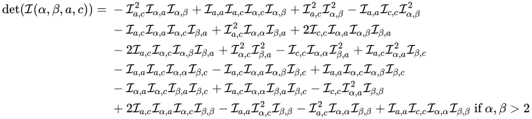
Using Sylvester's criterion (checking whether the diagonal elements are all positive), and since diagonal components and have singularities at α=2 and β=2 it follows that the Fisher information matrix for the four parameter case is positive-definite for α>2 and β>2. Since for α > 2 and β > 2 the beta distribution is (symmetric or unsymmetric) bell shaped, it follows that the Fisher information matrix is positive-definite only for bell-shaped (symmetric or unsymmetric) beta distributions, with inflection points located to either side of the mode. Thus, important well known distributions belonging to the four-parameter beta distribution family, like the parabolic distribution (Beta(2,2,a,c)) and the uniform distribution (Beta(1,1,a,c)) have Fisher information components () that blow up (approach infinity) in the four-parameter case (although their Fisher information components are all defined for the two parameter case). The four-parameter Wigner semicircle distribution (Beta(3/2,3/2,a,c)) and arcsine distribution (Beta(1/2,1/2,a,c)) have negative Fisher information determinants for the four-parameter case.

Bayesian inference


The use of Beta distributions in Bayesian inference is due to the fact that they provide a family of conjugate prior probability distributions for binomial (including Bernoulli) and geometric distributions. The domain of the beta distribution can be viewed as a probability, and in fact the beta distribution is often used to describe the distribution of a probability value p:[24]
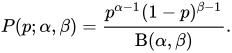
Examples of beta distributions used as prior probabilities to represent ignorance of prior parameter values in Bayesian inference are Beta(1,1), Beta(0,0) and Beta(1/2,1/2).
Rule of succession
A classic application of the beta distribution is the rule of succession, introduced in the 18th century by Pierre-Simon Laplace[56] in the course of treating the sunrise problem. It states that, given s successes in nconditionally independentBernoulli trials with probability p, that the estimate of the expected value in the next trial is . This estimate is the expected value of the posterior distribution over p, namely Beta(s+1, n−s+1), which is given by Bayes' rule if one assumes a uniform prior probability over p (i.e., Beta(1, 1)) and then observes that p generated s successes in n trials. Laplace's rule of succession has been criticized by prominent scientists. R. T. Cox described Laplace's application of the rule of succession to the sunrise problem ([57] p. 89) as "a travesty of the proper use of the principle". Keynes remarks ([58] Ch.XXX, p. 382) "indeed this is so foolish a theorem that to entertain it is discreditable". Karl Pearson[59] showed that the probability that the next (n + 1) trials will be successes, after n successes in n trials, is only 50%, which has been considered too low by scientists like Jeffreys and unacceptable as a representation of the scientific process of experimentation to test a proposed scientific law. As pointed out by Jeffreys ([60] p. 128) (crediting C. D. Broad[61] ) Laplace's rule of succession establishes a high probability of success ((n+1)/(n+2)) in the next trial, but only a moderate probability (50%) that a further sample (n+1) comparable in size will be equally successful. As pointed out by Perks,[62] "The rule of succession itself is hard to accept. It assigns a probability to the next trial which implies the assumption that the actual run observed is an average run and that we are always at the end of an average run. It would, one would think, be more reasonable to assume that we were in the middle of an average run. Clearly a higher value for both probabilities is necessary if they are to accord with reasonable belief." These problems with Laplace's rule of succession motivated Haldane, Perks, Jeffreys and others to search for other forms of prior probability (see the next § Bayesian inference). According to Jaynes,[53] the main problem with the rule of succession is that it is not valid when s=0 or s=n (see rule of succession, for an analysis of its validity).

Bayes–Laplace prior probability (Beta(1,1))
The beta distribution achieves maximum differential entropy for Beta(1,1): the uniform probability density, for which all values in the domain of the distribution have equal density. This uniform distribution Beta(1,1) was suggested ("with a great deal of doubt") by Thomas Bayes[63] as the prior probability distribution to express ignorance about the correct prior distribution. This prior distribution was adopted (apparently, from his writings, with little sign of doubt[56]) by Pierre-Simon Laplace, and hence it was also known as the "Bayes–Laplace rule" or the "Laplace rule" of "inverse probability" in publications of the first half of the 20th century. In the later part of the 19th century and early part of the 20th century, scientists realized that the assumption of uniform "equal" probability density depended on the actual functions (for example whether a linear or a logarithmic scale was most appropriate) and parametrizations used. In particular, the behavior near the ends of distributions with finite support (for example near x = 0, for a distribution with initial support at x = 0) required particular attention. Keynes ([58] Ch.XXX, p. 381) criticized the use of Bayes's uniform prior probability (Beta(1,1)) that all values between zero and one are equiprobable, as follows: "Thus experience, if it shows anything, shows that there is a very marked clustering of statistical ratios in the neighborhoods of zero and unity, of those for positive theories and for correlations between positive qualities in the neighborhood of zero, and of those for negative theories and for correlations between negative qualities in the neighborhood of unity. "
Haldane's prior probability (Beta(0,0))


The Beta(0,0) distribution was proposed by J.B.S. Haldane,[64] who suggested that the prior probability representing complete uncertainty should be proportional to p−1(1−p)−1. The function p−1(1−p)−1 can be viewed as the limit of the numerator of the beta distribution as both shape parameters approach zero: α, β → 0. The Beta function (in the denominator of the beta distribution) approaches infinity, for both parameters approaching zero, α, β → 0. Therefore, p−1(1−p)−1 divided by the Beta function approaches a 2-point Bernoulli distribution with equal probability 1/2 at each end, at 0 and 1, and nothing in between, as α, β → 0. A coin-toss: one face of the coin being at 0 and the other face being at 1. The Haldane prior probability distribution Beta(0,0) is an "improper prior" because its integration (from 0 to 1) fails to strictly converge to 1 due to the singularities at each end. However, this is not an issue for computing posterior probabilities unless the sample size is very small. Furthermore, Zellner[65] points out that on the log-odds scale, (the logit transformation ), the Haldane prior is the uniformly flat prior. The fact that a uniform prior probability on the logit transformed variable ln(p/1 − p) (with domain (−∞, ∞)) is equivalent to the Haldane prior on the domain [0, 1] was pointed out by Harold Jeffreys in the first edition (1939) of his book Theory of Probability ([60] p. 123). Jeffreys writes "Certainly if we take the Bayes–Laplace rule right up to the extremes we are led to results that do not correspond to anybody's way of thinking. The (Haldane) rule dx/(x(1 − x)) goes too far the other way. It would lead to the conclusion that if a sample is of one type with respect to some property there is a probability 1 that the whole population is of that type." The fact that "uniform" depends on the parametrization, led Jeffreys to seek a form of prior that would be invariant under different parametrizations.

Jeffreys' prior probability (Beta(1/2,1/2) for a Bernoulli or for a binomial distribution)




Harold Jeffreys[60][66] proposed to use an uninformative prior probability measure that should be invariant under reparameterization: proportional to the square root of the determinant of Fisher's information matrix. For the Bernoulli distribution, this can be shown as follows: for a coin that is "heads" with probability p ∈ [0, 1] and is "tails" with probability 1 − p, for a given (H,T) ∈ {(0,1), (1,0)} the probability is pH(1 − p)T. Since T = 1 − H, the Bernoulli distribution is pH(1 − p)1 − H. Considering p as the only parameter, it follows that the log likelihood for the Bernoulli distribution is

The Fisher information matrix has only one component (it is a scalar, because there is only one parameter: p), therefore:
![{\displaystyle {\begin{aligned}{\sqrt {{\mathcal {I}}(p)}}&={\sqrt {\operatorname {E} \!\left[\left({\frac {d}{dp}}\ln {\mathcal {L}}(p\mid H)\right)^{2}\right]}}\\[6pt]&={\sqrt {\operatorname {E} \!\left[\left({\frac {H}{p}}-{\frac {1-H}{1-p}}\right)^{2}\right]}}\\[6pt]&={\sqrt {p^{1}(1-p)^{0}\left({\frac {1}{p}}-{\frac {0}{1-p}}\right)^{2}+p^{0}(1-p)^{1}\left({\frac {0}{p}}-{\frac {1}{1-p}}\right)^{2}}}\\&={\frac {1}{\sqrt {p(1-p)}}}.\end{aligned}}}](https://wikimedia.org/api/rest_v1/media/math/render/svg/0c2541cc4a3017abaab79170bd990ca92a64bc89)
Similarly, for the Binomial distribution with nBernoulli trials, it can be shown that

Thus, for the Bernoulli, and Binomial distributions, Jeffreys prior is proportional to , which happens to be proportional to a beta distribution with domain variable x = p, and shape parameters α = β = 1/2, the arcsine distribution:


It will be shown in the next section that the normalizing constant for Jeffreys prior is immaterial to the final result because the normalizing constant cancels out in Bayes' theorem for the posterior probability. Hence Beta(1/2,1/2) is used as the Jeffreys prior for both Bernoulli and binomial distributions. As shown in the next section, when using this expression as a prior probability times the likelihood in Bayes' theorem, the posterior probability turns out to be a beta distribution. It is important to realize, however, that Jeffreys prior is proportional to for the Bernoulli and binomial distribution, but not for the beta distribution. Jeffreys prior for the beta distribution is given by the determinant of Fisher's information for the beta distribution, which, as shown in the § Fisher information matrix is a function of the trigamma function ψ1 of shape parameters α and β as follows:

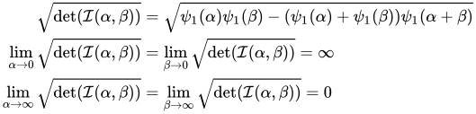
As previously discussed, Jeffreys prior for the Bernoulli and binomial distributions is proportional to the arcsine distribution Beta(1/2,1/2), a one-dimensional curve that looks like a basin as a function of the parameter p of the Bernoulli and binomial distributions. The walls of the basin are formed by p approaching the singularities at the ends p → 0 and p → 1, where Beta(1/2,1/2) approaches infinity. Jeffreys prior for the beta distribution is a 2-dimensional surface (embedded in a three-dimensional space) that looks like a basin with only two of its walls meeting at the corner α = β = 0 (and missing the other two walls) as a function of the shape parameters α and β of the beta distribution. The two adjoining walls of this 2-dimensional surface are formed by the shape parameters α and β approaching the singularities (of the trigamma function) at α, β → 0. It has no walls for α, β → ∞ because in this case the determinant of Fisher's information matrix for the beta distribution approaches zero.
It will be shown in the next section that Jeffreys prior probability results in posterior probabilities (when multiplied by the binomial likelihood function) that are intermediate between the posterior probability results of the Haldane and Bayes prior probabilities.
Jeffreys prior may be difficult to obtain analytically, and for some cases it just doesn't exist (even for simple distribution functions like the asymmetric triangular distribution). Berger, Bernardo and Sun, in a 2009 paper[67] defined a reference prior probability distribution that (unlike Jeffreys prior) exists for the asymmetric triangular distribution. They cannot obtain a closed-form expression for their reference prior, but numerical calculations show it to be nearly perfectly fitted by the (proper) prior
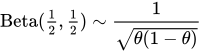
where θ is the vertex variable for the asymmetric triangular distribution with support [0, 1] (corresponding to the following parameter values in Wikipedia's article on the triangular distribution: vertex c = θ, left end a = 0, and right end b = 1). Berger et al. also give a heuristic argument that Beta(1/2,1/2) could indeed be the exact Berger–Bernardo–Sun reference prior for the asymmetric triangular distribution. Therefore, Beta(1/2,1/2) not only is Jeffreys prior for the Bernoulli and binomial distributions, but also seems to be the Berger–Bernardo–Sun reference prior for the asymmetric triangular distribution (for which the Jeffreys prior does not exist), a distribution used in project management and PERT analysis to describe the cost and duration of project tasks.
Clarke and Barron[68] prove that, among continuous positive priors, Jeffreys prior (when it exists) asymptotically maximizes Shannon's mutual information between a sample of size n and the parameter, and therefore Jeffreys prior is the most uninformative prior (measuring information as Shannon information). The proof rests on an examination of the Kullback–Leibler divergence between probability density functions for iid random variables.
Effect of different prior probability choices on the posterior beta distribution
If samples are drawn from the population of a random variable X that result in s successes and f failures in nBernoulli trialsn = s + f, then the likelihood function for parameters s and f given x = p (the notation x = p in the expressions below will emphasize that the domain x stands for the value of the parameter p in the binomial distribution), is the following binomial distribution:

If beliefs about prior probability information are reasonably well approximated by a beta distribution with parameters α Prior and β Prior, then:

According to Bayes' theorem for a continuous event space, the posterior probability density is given by the product of the prior probability and the likelihood function (given the evidence s and f = n − s), normalized so that the area under the curve equals one, as follows:
![{\displaystyle {\begin{aligned}&{\text{posterior probability density}}(x=p\mid s,n-s)\\[6pt]={}&{\frac {\operatorname {priorprobabilitydensity} (x=p;\alpha \operatorname {prior} ,\beta \operatorname {prior} ){\mathcal {L}}(s,f\mid x=p)}{\int _{0}^{1}{\text{prior probability density}}(x=p;\alpha \operatorname {prior} ,\beta \operatorname {prior} ){\mathcal {L}}(s,f\mid x=p)\,dx}}\\[6pt]={}&{\frac {{n \choose s}x^{s+\alpha \operatorname {prior} -1}(1-x)^{n-s+\beta \operatorname {prior} -1}/\mathrm {B} (\alpha \operatorname {prior} ,\beta \operatorname {prior} )}{\int _{0}^{1}\left({n \choose s}x^{s+\alpha \operatorname {prior} -1}(1-x)^{n-s+\beta \operatorname {prior} -1}/\mathrm {B} (\alpha \operatorname {prior} ,\beta \operatorname {prior} )\right)\,dx}}\\[6pt]={}&{\frac {x^{s+\alpha \operatorname {prior} -1}(1-x)^{n-s+\beta \operatorname {prior} -1}}{\int _{0}^{1}\left(x^{s+\alpha \operatorname {prior} -1}(1-x)^{n-s+\beta \operatorname {prior} -1}\right)\,dx}}\\[6pt]={}&{\frac {x^{s+\alpha \operatorname {prior} -1}(1-x)^{n-s+\beta \operatorname {prior} -1}}{\mathrm {B} (s+\alpha \operatorname {prior} ,n-s+\beta \operatorname {prior} )}}.\end{aligned}}}](https://wikimedia.org/api/rest_v1/media/math/render/svg/569ad0317cf545ff98538c8a845f216120e87c08)

appears both in the numerator and the denominator of the posterior probability, and it does not depend on the integration variable x, hence it cancels out, and it is irrelevant to the final result. Similarly the normalizing factor for the prior probability, the beta function B(αPrior,βPrior) cancels out and it is immaterial to the final result. The same posterior probability result can be obtained if one uses an un-normalized prior

because the normalizing factors all cancel out. Several authors (including Jeffreys himself) thus use an un-normalized prior formula since the normalization constant cancels out. The numerator of the posterior probability ends up being just the (un-normalized) product of the prior probability and the likelihood function, and the denominator is its integral from zero to one. The beta function in the denominator, B(s + α Prior, n − s + β Prior), appears as a normalization constant to ensure that the total posterior probability integrates to unity.
The ratio s/n of the number of successes to the total number of trials is a sufficient statistic in the binomial case, which is relevant for the following results.
For the Bayes' prior probability (Beta(1,1)), the posterior probability is:

For the Jeffreys' prior probability (Beta(1/2,1/2)), the posterior probability is:

and for the Haldane prior probability (Beta(0,0)), the posterior probability is:

From the above expressions it follows that for s/n = 1/2) all the above three prior probabilities result in the identical location for the posterior probability mean = mode = 1/2. For s/n < 1/2, the mean of the posterior probabilities, using the following priors, are such that: mean for Bayes prior > mean for Jeffreys prior > mean for Haldane prior. For s/n > 1/2 the order of these inequalities is reversed such that the Haldane prior probability results in the largest posterior mean. The Haldane prior probability Beta(0,0) results in a posterior probability density with mean (the expected value for the probability of success in the "next" trial) identical to the ratio s/n of the number of successes to the total number of trials. Therefore, the Haldane prior results in a posterior probability with expected value in the next trial equal to the maximum likelihood. The Bayes prior probability Beta(1,1) results in a posterior probability density with mode identical to the ratio s/n (the maximum likelihood).
In the case that 100% of the trials have been successful s = n, the Bayes prior probability Beta(1,1) results in a posterior expected value equal to the rule of succession (n + 1)/(n + 2), while the Haldane prior Beta(0,0) results in a posterior expected value of 1 (absolute certainty of success in the next trial). Jeffreys prior probability results in a posterior expected value equal to (n + 1/2)/(n + 1). Perks[62] (p. 303) points out: "This provides a new rule of succession and expresses a 'reasonable' position to take up, namely, that after an unbroken run of n successes we assume a probability for the next trial equivalent to the assumption that we are about half-way through an average run, i.e. that we expect a failure once in (2n + 2) trials. The Bayes–Laplace rule implies that we are about at the end of an average run or that we expect a failure once in (n + 2) trials. The comparison clearly favours the new result (what is now called Jeffreys prior) from the point of view of 'reasonableness'."
Conversely, in the case that 100% of the trials have resulted in failure (s = 0), the Bayes prior probability Beta(1,1) results in a posterior expected value for success in the next trial equal to 1/(n + 2), while the Haldane prior Beta(0,0) results in a posterior expected value of success in the next trial of 0 (absolute certainty of failure in the next trial). Jeffreys prior probability results in a posterior expected value for success in the next trial equal to (1/2)/(n + 1), which Perks[62] (p. 303) points out: "is a much more reasonably remote result than the Bayes–Laplace result 1/(n + 2)".
Jaynes[53] questions (for the Haldane prior Beta(0,0)) the use of these formulas for the cases s = 0 or s = n because the integrals do not converge (Beta(0,0) is an improper prior for s = 0 or s = n). In practice, the conditions 0<s<n necessary for a mode to exist between both ends for the Bayes prior are usually met, and therefore the Bayes prior (as long as 0 < s < n) results in a posterior mode located between both ends of the domain.
As remarked in the section on the rule of succession, K. Pearson showed that after n successes in n trials the posterior probability (based on the Bayes Beta(1,1) distribution as the prior probability) that the next (n + 1) trials will all be successes is exactly 1/2, whatever the value of n. Based on the Haldane Beta(0,0) distribution as the prior probability, this posterior probability is 1 (absolute certainty that after n successes in n trials the next (n + 1) trials will all be successes). Perks[62] (p. 303) shows that, for what is now known as the Jeffreys prior, this probability is ((n + 1/2)/(n + 1))((n + 3/2)/(n + 2))...(2n + 1/2)/(2n + 1), which for n = 1, 2, 3 gives 15/24, 315/480, 9009/13440; rapidly approaching a limiting value of as n tends to infinity. Perks remarks that what is now known as the Jeffreys prior: "is clearly more 'reasonable' than either the Bayes–Laplace result or the result on the (Haldane) alternative rule rejected by Jeffreys which gives certainty as the probability. It clearly provides a very much better correspondence with the process of induction. Whether it is 'absolutely' reasonable for the purpose, i.e. whether it is yet large enough, without the absurdity of reaching unity, is a matter for others to decide. But it must be realized that the result depends on the assumption of complete indifference and absence of knowledge prior to the sampling experiment."

Following are the variances of the posterior distribution obtained with these three prior probability distributions:
for the Bayes' prior probability (Beta(1,1)), the posterior variance is:

for the Jeffreys' prior probability (Beta(1/2,1/2)), the posterior variance is:

and for the Haldane prior probability (Beta(0,0)), the posterior variance is:

So, as remarked by Silvey,[51] for large n, the variance is small and hence the posterior distribution is highly concentrated, whereas the assumed prior distribution was very diffuse. This is in accord with what one would hope for, as vague prior knowledge is transformed (through Bayes' theorem) into a more precise posterior knowledge by an informative experiment. For small n the Haldane Beta(0,0) prior results in the largest posterior variance while the Bayes Beta(1,1) prior results in the more concentrated posterior. Jeffreys prior Beta(1/2,1/2) results in a posterior variance in between the other two. As n increases, the variance rapidly decreases so that the posterior variance for all three priors converges to approximately the same value (approaching zero variance as n → ∞). Recalling the previous result that the Haldane prior probability Beta(0,0) results in a posterior probability density with mean (the expected value for the probability of success in the "next" trial) identical to the ratio s/n of the number of successes to the total number of trials, it follows from the above expression that also the Haldane prior Beta(0,0) results in a posterior with variance identical to the variance expressed in terms of the max. likelihood estimate s/n and sample size (in § Variance):

with the mean μ = s/n and the sample size ν = n.
In Bayesian inference, using a prior distribution Beta(αPrior,βPrior) prior to a binomial distribution is equivalent to adding (αPrior − 1) pseudo-observations of "success" and (βPrior − 1) pseudo-observations of "failure" to the actual number of successes and failures observed, then estimating the parameter p of the binomial distribution by the proportion of successes over both real- and pseudo-observations. A uniform prior Beta(1,1) does not add (or subtract) any pseudo-observations since for Beta(1,1) it follows that (αPrior − 1) = 0 and (βPrior − 1) = 0. The Haldane prior Beta(0,0) subtracts one pseudo observation from each and Jeffreys prior Beta(1/2,1/2) subtracts 1/2 pseudo-observation of success and an equal number of failure. This subtraction has the effect of smoothing out the posterior distribution. If the proportion of successes is not 50% (s/n ≠ 1/2) values of αPrior and βPrior less than 1 (and therefore negative (αPrior − 1) and (βPrior − 1)) favor sparsity, i.e. distributions where the parameter p is closer to either 0 or 1. In effect, values of αPrior and βPrior between 0 and 1, when operating together, function as a concentration parameter.
The accompanying plots show the posterior probability density functions for sample sizes n ∈ {3,10,50}, successes s ∈ {n/2,n/4} and Beta(αPrior,βPrior) ∈ {Beta(0,0),Beta(1/2,1/2),Beta(1,1)}. Also shown are the cases for n = {4,12,40}, success s = {n/4} and Beta(αPrior,βPrior) ∈ {Beta(0,0),Beta(1/2,1/2),Beta(1,1)}. The first plot shows the symmetric cases, for successes s ∈ {n/2}, with mean = mode = 1/2 and the second plot shows the skewed cases s ∈ {n/4}. The images show that there is little difference between the priors for the posterior with sample size of 50 (characterized by a more pronounced peak near p = 1/2). Significant differences appear for very small sample sizes (in particular for the flatter distribution for the degenerate case of sample size = 3). Therefore, the skewed cases, with successes s = {n/4}, show a larger effect from the choice of prior, at small sample size, than the symmetric cases. For symmetric distributions, the Bayes prior Beta(1,1) results in the most "peaky" and highest posterior distributions and the Haldane prior Beta(0,0) results in the flattest and lowest peak distribution. The Jeffreys prior Beta(1/2,1/2) lies in between them. For nearly symmetric, not too skewed distributions the effect of the priors is similar. For very small sample size (in this case for a sample size of 3) and skewed distribution (in this example for s ∈ {n/4}) the Haldane prior can result in a reverse-J-shaped distribution with a singularity at the left end. However, this happens only in degenerate cases (in this example n = 3 and hence s = 3/4 < 1, a degenerate value because s should be greater than unity in order for the posterior of the Haldane prior to have a mode located between the ends, and because s = 3/4 is not an integer number, hence it violates the initial assumption of a binomial distribution for the likelihood) and it is not an issue in generic cases of reasonable sample size (such that the condition 1 < s < n − 1, necessary for a mode to exist between both ends, is fulfilled).
In Chapter 12 (p. 385) of his book, Jaynes[53] asserts that the Haldane prior Beta(0,0) describes a prior state of knowledge of complete ignorance, where we are not even sure whether it is physically possible for an experiment to yield either a success or a failure, while the Bayes (uniform) prior Beta(1,1) applies if one knows that both binary outcomes are possible. Jaynes states: "interpret the Bayes–Laplace (Beta(1,1)) prior as describing not a state of complete ignorance, but the state of knowledge in which we have observed one success and one failure...once we have seen at least one success and one failure, then we know that the experiment is a true binary one, in the sense of physical possibility." Jaynes [53] does not specifically discuss Jeffreys prior Beta(1/2,1/2) (Jaynes discussion of "Jeffreys prior" on pp. 181, 423 and on chapter 12 of Jaynes book[53] refers instead to the improper, un-normalized, prior "1/p dp" introduced by Jeffreys in the 1939 edition of his book,[60] seven years before he introduced what is now known as Jeffreys' invariant prior: the square root of the determinant of Fisher's information matrix. "1/p" is Jeffreys' (1946) invariant prior for the exponential distribution, not for the Bernoulli or binomial distributions). However, it follows from the above discussion that Jeffreys Beta(1/2,1/2) prior represents a state of knowledge in between the Haldane Beta(0,0) and Bayes Beta (1,1) prior.
Similarly, Karl Pearson in his 1892 book The Grammar of Science[69][70] (p. 144 of 1900 edition) maintained that the Bayes (Beta(1,1) uniform prior was not a complete ignorance prior, and that it should be used when prior information justified to "distribute our ignorance equally"". K. Pearson wrote: "Yet the only supposition that we appear to have made is this: that, knowing nothing of nature, routine and anomy (from the Greek ανομία, namely: a- "without", and nomos "law") are to be considered as equally likely to occur. Now we were not really justified in making even this assumption, for it involves a knowledge that we do not possess regarding nature. We use our experience of the constitution and action of coins in general to assert that heads and tails are equally probable, but we have no right to assert before experience that, as we know nothing of nature, routine and breach are equally probable. In our ignorance we ought to consider before experience that nature may consist of all routines, all anomies (normlessness), or a mixture of the two in any proportion whatever, and that all such are equally probable. Which of these constitutions after experience is the most probable must clearly depend on what that experience has been like."
If there is sufficient sampling data, and the posterior probability mode is not located at one of the extremes of the domain (x = 0 or x = 1), the three priors of Bayes (Beta(1,1)), Jeffreys (Beta(1/2,1/2)) and Haldane (Beta(0,0)) should yield similar posterior probability densities. Otherwise, as Gelman et al.[71] (p. 65) point out, "if so few data are available that the choice of noninformative prior distribution makes a difference, one should put relevant information into the prior distribution", or as Berger[4] (p. 125) points out "when different reasonable priors yield substantially different answers, can it be right to state that there is a single answer? Would it not be better to admit that there is scientific uncertainty, with the conclusion depending on prior beliefs?."
Occurrence and applications
Order statistics
The beta distribution has an important application in the theory of order statistics. A basic result is that the distribution of the kth smallest of a sample of size n from a continuous uniform distribution has a beta distribution.[40] This result is summarized as

From this, and application of the theory related to the probability integral transform, the distribution of any individual order statistic from any continuous distribution can be derived.[40]
Subjective logic
In standard logic, propositions are considered to be either true or false. In contradistinction, subjective logic assumes that humans cannot determine with absolute certainty whether a proposition about the real world is absolutely true or false. In subjective logic the posteriori probability estimates of binary events can be represented by beta distributions.[72]
Wavelet analysis
A wavelet is a wave-like oscillation with an amplitude that starts out at zero, increases, and then decreases back to zero. It can typically be visualized as a "brief oscillation" that promptly decays. Wavelets can be used to extract information from many different kinds of data, including – but certainly not limited to – audio signals and images. Thus, wavelets are purposefully crafted to have specific properties that make them useful for signal processing. Wavelets are localized in both time and frequency whereas the standard Fourier transform is only localized in frequency. Therefore, standard Fourier Transforms are only applicable to stationary processes, while wavelets are applicable to non-stationary processes. Continuous wavelets can be constructed based on the beta distribution. Beta wavelets[73] can be viewed as a soft variety of Haar wavelets whose shape is fine-tuned by two shape parameters α and β.
Population genetics
The Balding–Nichols model is a two-parameter parametrization of the beta distribution used in population genetics.[74] It is a statistical description of the allele frequencies in the components of a sub-divided population:
where and ; here F is (Wright's) genetic distance between two populations.
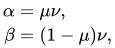
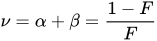

Project management: task cost and schedule modeling
The beta distribution can be used to model events which are constrained to take place within an interval defined by a minimum and maximum value. For this reason, the beta distribution — along with the triangular distribution — is used extensively in PERT, critical path method (CPM), Joint Cost Schedule Modeling (JCSM) and other project management/control systems to describe the time to completion and the cost of a task. In project management, shorthand computations are widely used to estimate the mean and standard deviation of the beta distribution:[39]
![{\displaystyle {\begin{aligned}\mu (X)&={\frac {a+4b+c}{6}}\\[8pt]\sigma (X)&={\frac {c-a}{6}}\end{aligned}}}](https://wikimedia.org/api/rest_v1/media/math/render/svg/7a89a68d1250ebe659be15e88edb5a9eb3e0cf87)
where a is the minimum, c is the maximum, and b is the most likely value (the mode for α > 1 and β > 1).
The above estimate for the mean is known as the PERTthree-point estimation and it is exact for either of the following values of β (for arbitrary α within these ranges):
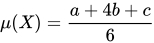
- β = α > 1 (symmetric case) with standard deviation, skewness = 0, and excess kurtosis =
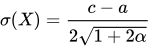


or
- β = 6 − α for 5 > α > 1 (skewed case) with standard deviation
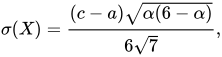
skewness, and excess kurtosis
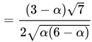
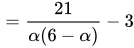

The above estimate for the standard deviationσ(X) = (c − a)/6 is exact for either of the following values of α and β:
- α = β = 4 (symmetric) with skewness = 0, and excess kurtosis = −6/11.
- β = 6 − α and (right-tailed, positive skew) with skewness, and excess kurtosis = 0
- β = 6 − α and (left-tailed, negative skew) with skewness, and excess kurtosis = 0


Otherwise, these can be poor approximations for beta distributions with other values of α and β, exhibiting average errors of 40% in the mean and 549% in the variance.[75][76][77]
Random variate generation
If X and Y are independent, with and then


So one algorithm for generating beta variates is to generate , where X is a gamma variate with parameters (α, 1) and Y is an independent gamma variate with parameters (β, 1).[78] In fact, here and are independent, and . If and is independent of and , then and is independent of . This shows that the product of independent and random variables is a random variable.





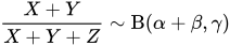


Also, the kth order statistic of nuniformly distributed variates is , so an alternative if α and β are small integers is to generate α + β − 1 uniform variates and choose the α-th smallest.[40]

Another way to generate the Beta distribution is by Pólya urn model. According to this method, one starts with an "urn" with α "black" balls and β "white" balls and draws uniformly with replacement. Every trial an additional ball is added according to the color of the last ball which was drawn. Asymptotically, the proportion of black and white balls will be distributed according to the Beta distribution, where each repetition of the experiment will produce a different value.
It is also possible to use the inverse transform sampling.
Normal approximation to the Beta distribution
A beta distribution with and and is approximately normal with mean and variance . If the normal approximation can be improved by taking the cube-root of the logarithm of the reciprocal of [79][80]


History
Thomas Bayes, in a posthumous paper [63] published in 1763 by Richard Price, obtained a beta distribution as the density of the probability of success in Bernoulli trials (see § Applications, Bayesian inference), but the paper does not analyze any of the moments of the beta distribution or discuss any of its properties.

The first systematic modern discussion of the beta distribution is probably due to Karl Pearson.[81][82] In Pearson's papers[21][33] the beta distribution is couched as a solution of a differential equation: Pearson's Type I distribution which it is essentially identical to except for arbitrary shifting and re-scaling (the beta and Pearson Type I distributions can always be equalized by proper choice of parameters). In fact, in several English books and journal articles in the few decades prior to World War II, it was common to refer to the beta distribution as Pearson's Type I distribution. William P. Elderton in his 1906 monograph "Frequency curves and correlation"[43] further analyzes the beta distribution as Pearson's Type I distribution, including a full discussion of the method of moments for the four parameter case, and diagrams of (what Elderton describes as) U-shaped, J-shaped, twisted J-shaped, "cocked-hat" shapes, horizontal and angled straight-line cases. Elderton wrote "I am chiefly indebted to Professor Pearson, but the indebtedness is of a kind for which it is impossible to offer formal thanks." Elderton in his 1906 monograph [43] provides an impressive amount of information on the beta distribution, including equations for the origin of the distribution chosen to be the mode, as well as for other Pearson distributions: types I through VII. Elderton also included a number of appendixes, including one appendix ("II") on the beta and gamma functions. In later editions, Elderton added equations for the origin of the distribution chosen to be the mean, and analysis of Pearson distributions VIII through XII.
As remarked by Bowman and Shenton[45] "Fisher and Pearson had a difference of opinion in the approach to (parameter) estimation, in particular relating to (Pearson's method of) moments and (Fisher's method of) maximum likelihood in the case of the Beta distribution." Also according to Bowman and Shenton, "the case of a Type I (beta distribution) model being the center of the controversy was pure serendipity. A more difficult model of 4 parameters would have been hard to find." The long running public conflict of Fisher with Karl Pearson can be followed in a number of articles in prestigious journals. For example, concerning the estimation of the four parameters for the beta distribution, and Fisher's criticism of Pearson's method of moments as being arbitrary, see Pearson's article "Method of moments and method of maximum likelihood" [46] (published three years after his retirement from University College, London, where his position had been divided between Fisher and Pearson's son Egon) in which Pearson writes "I read (Koshai's paper in the Journal of the Royal Statistical Society, 1933) which as far as I am aware is the only case at present published of the application of Professor Fisher's method. To my astonishment that method depends on first working out the constants of the frequency curve by the (Pearson) Method of Moments and then superposing on it, by what Fisher terms "the Method of Maximum Likelihood" a further approximation to obtain, what he holds, he will thus get, 'more efficient values' of the curve constants".
David and Edwards's treatise on the history of statistics[83] cites the first modern treatment of the beta distribution, in 1911,[84] using the beta designation that has become standard, due to Corrado Gini, an Italian statistician, demographer, and sociologist, who developed the Gini coefficient. N.L.Johnson and S.Kotz, in their comprehensive and very informative monograph[85] on leading historical personalities in statistical sciences credit Corrado Gini[86] as "an early Bayesian...who dealt with the problem of eliciting the parameters of an initial Beta distribution, by singling out techniques which anticipated the advent of the so-called empirical Bayes approach."
References
- 12345678910111213141516171819202122232425Johnson, Norman L.; Kotz, Samuel; Balakrishnan, N. (1995). "Chapter 25: Beta Distributions". Continuous Univariate Distributions Vol. 2 (2nd ed.). Wiley. ISBN 978-0-471-58494-0.
- 12Rose, Colin; Smith, Murray D. (2002). Mathematical Statistics with MATHEMATICA. Springer. ISBN 978-0387952345.
- 123Kruschke, John K. (2011). Doing Bayesian data analysis: A tutorial with R and BUGS. Academic Press / Elsevier. p. 83. ISBN 978-0123814852.
- 12Berger, James O. (2010). Statistical Decision Theory and Bayesian Analysis (2nd ed.). Springer. ISBN 978-1441930743.
- 123Feller, William (1971). An Introduction to Probability Theory and Its Applications, Vol. 2. Wiley. ISBN 978-0471257097.
- ↑Wadsworth, G. P. (1960). Introduction to Probability and Random Variables. New York: McGraw-Hill. p. 52.
- ↑Kruschke, John K. (2015). Doing Bayesian Data Analysis: A Tutorial with R, JAGS and Stan. Academic Press / Elsevier. ISBN 978-0-12-405888-0.
- 12Wadsworth, George P. and Joseph Bryan (1960). Introduction to Probability and Random Variables. McGraw-Hill.
- 1234567Gupta, Arjun K., ed. (2004). Handbook of Beta Distribution and Its Applications. CRC Press. ISBN 978-0824753962.
- 12Kerman, Jouni (2011). "A closed-form approximation for the median of the beta distribution". arXiv:1111.0433 [math.ST].
- ↑Mosteller, Frederick and John Tukey (1977). Data Analysis and Regression: A Second Course in Statistics. Addison-Wesley Pub. Co. Bibcode:1977dars.book.....M. ISBN 978-0201048544.
- ↑Feller, William (1968). An Introduction to Probability Theory and Its Applications. Vol. 1 (3rd ed.). Wiley. ISBN 978-0471257080.
- ↑Philip J. Fleming and John J. Wallace. How not to lie with statistics: the correct way to summarize benchmark results. Communications of the ACM, 29(3):218–221, March 1986.
- ↑"NIST/SEMATECH e-Handbook of Statistical Methods 1.3.6.6.17. Beta Distribution". National Institute of Standards and Technology Information Technology Laboratory. April 2012. Retrieved May 31, 2016.
- ↑Oguamanam, D.C.D.; Martin, H. R.; Huissoon, J. P. (1995). "On the application of the beta distribution to gear damage analysis". Applied Acoustics. 45 (3): 247–261. doi:10.1016/0003-682X(95)00001-P.
- ↑Zhiqiang Liang; Jianming Wei; Junyu Zhao; Haitao Liu; Baoqing Li; Jie Shen; Chunlei Zheng (27 August 2008). "The Statistical Meaning of Kurtosis and Its New Application to Identification of Persons Based on Seismic Signals". Sensors. 8 (8): 5106–5119. Bibcode:2008Senso...8.5106L. doi:10.3390/s8085106. PMC 3705491. PMID 27873804.
- ↑Kenney, J. F., and E. S. Keeping (1951). Mathematics of Statistics Part Two, 2nd edition. D. Van Nostrand Company Inc.
{{cite book}}: CS1 maint: multiple names: authors list (link) - 1234Abramowitz, Milton and Irene A. Stegun (1965). Handbook Of Mathematical Functions With Formulas, Graphs, And Mathematical Tables. Dover. ISBN 978-0-486-61272-0.
- ↑Weisstein., Eric W. "Kurtosis". MathWorld--A Wolfram Web Resource. Retrieved 13 August 2012.
- 12Panik, Michael J (2005). Advanced Statistics from an Elementary Point of View. Academic Press. ISBN 978-0120884940.
- 123456Pearson, Karl (1916). "Mathematical contributions to the theory of evolution, XIX: Second supplement to a memoir on skew variation". Philosophical Transactions of the Royal Society A. 216 (538–548): 429–457. Bibcode:1916RSPTA.216..429P. doi:10.1098/rsta.1916.0009. JSTOR 91092.
- ↑Gradshteyn, Izrail Solomonovich; Ryzhik, Iosif Moiseevich; Geronimus, Yuri Veniaminovich; Tseytlin, Michail Yulyevich; Jeffrey, Alan (2015) [October 2014]. Zwillinger, Daniel; Moll, Victor Hugo (eds.). Table of Integrals, Series, and Products. Translated by Scripta Technica, Inc. (8 ed.). Academic Press, Inc.ISBN 978-0-12-384933-5. LCCN 2014010276.
- ↑Billingsley, Patrick (1995). "Section 30: The Method of Moments". Probability and measure (3rd ed.). Wiley-Interscience. ISBN 978-0-471-00710-4.
- 12MacKay, David (2003). Information Theory, Inference and Learning Algorithms. Cambridge University Press; First Edition. Bibcode:2003itil.book.....M. ISBN 978-0521642989.
- 12Johnson, N.L. (1949). "Systems of frequency curves generated by methods of translation"(PDF). Biometrika. 36 (1–2): 149–176. doi:10.1093/biomet/36.1-2.149. hdl:10338.dmlcz/135506. PMID 18132090.
- ↑Verdugo Lazo, A. C. G.; Rathie, P. N. (1978). "On the entropy of continuous probability distributions". IEEE Trans. Inf. Theory. 24 (1): 120–122. doi:10.1109/TIT.1978.1055832.
- ↑Shannon, Claude E. (1948). "A Mathematical Theory of Communication". Bell System Technical Journal. 27 (4): 623–656. doi:10.1002/j.1538-7305.1948.tb01338.x.
- 123Cover, Thomas M. and Joy A. Thomas (2006). Elements of Information Theory 2nd Edition (Wiley Series in Telecommunications and Signal Processing). Wiley-Interscience; 2 edition. ISBN 978-0471241959.
- ↑Plunkett, Kim, and Jeffrey Elman (1997). Exercises in Rethinking Innateness: A Handbook for Connectionist Simulations (Neural Network Modeling and Connectionism). A Bradford Book. p. 166. ISBN 978-0262661058.
{{cite book}}: CS1 maint: multiple names: authors list (link) - ↑Nallapati, Ramesh (2006). The smoothed dirichlet distribution: understanding cross-entropy ranking in information retrieval (Thesis). Computer Science Dept., University of Massachusetts Amherst.
- 12Pearson, Egon S. (July 1969). "Some historical reflections traced through the development of the use of frequency curves". THEMIS Statistical Analysis Research Program, Technical Report 38. Office of Naval Research, Contract N000014-68-A-0515 (Project NR 042–260).
- ↑Hahn, Gerald J.; Shapiro, S. (1994). Statistical Models in Engineering (Wiley Classics Library). Wiley-Interscience. ISBN 978-0471040651.
- 12Pearson, Karl (1895). "Contributions to the mathematical theory of evolution, II: Skew variation in homogeneous material". Philosophical Transactions of the Royal Society. 186: 343–414. Bibcode:1895RSPTA.186..343P. doi:10.1098/rsta.1895.0010. JSTOR 90649.
- ↑Buchanan, K.; Rockway, J.; Sternberg, O.; Mai, N. N. (May 2016). "Sum-difference beamforming for radar applications using circularly tapered random arrays". 2016 IEEE Radar Conference (RadarConf). pp. 1–5. doi:10.1109/RADAR.2016.7485289. ISBN 978-1-5090-0863-6. S2CID 32525626.
- ↑Buchanan, K.; Flores, C.; Wheeland, S.; Jensen, J.; Grayson, D.; Huff, G. (May 2017). "Transmit beamforming for radar applications using circularly tapered random arrays". 2017 IEEE Radar Conference (RadarConf). pp. 0112–0117. doi:10.1109/RADAR.2017.7944181. ISBN 978-1-4673-8823-8. S2CID 38429370.
- ↑Ryan, Buchanan, Kristopher (2014-05-29). "Theory and Applications of Aperiodic (Random) Phased Arrays".
{{cite web}}: CS1 maint: multiple names: authors list (link) - ↑Pham-Gia, T. (January 2000). "Distributions of the ratios of independent beta variables and applications". Communications in Statistics - Theory and Methods. 29 (12): 2693–2715. doi:10.1080/03610920008832632. ISSN 0361-0926. Retrieved 13 November 2024.
- ↑Herrerías-Velasco, José Manuel and Herrerías-Pleguezuelo, Rafael and René van Dorp, Johan. (2011). Revisiting the PERT mean and Variance. European Journal of Operational Research (210), p. 448–451.
- 12Malcolm, D. G.; Roseboom, J. H.; Clark, C. E.; Fazar, W. (September–October 1958). "Application of a Technique for Research and Development Program Evaluation". Operations Research. 7 (5): 646–669. doi:10.1287/opre.7.5.646. ISSN 0030-364X.
- 1234David, H. A., Nagaraja, H. N. (2003) Order Statistics (3rd Edition). Wiley, New Jersey pp 458. ISBN 0-471-38926-9
- ↑Lee, Changwoo J.; Zito, Alessandro; Sang, Huiyan; Dunson, David B. (2025-12-01). "Logistic-Beta Processes for Dependent Random Probabilities with Beta Marginals". Bayesian Analysis. 20 (4). doi:10.1214/25-ba1541. ISSN 1936-0975.
- ↑"1.3.6.6.17. Beta Distribution". www.itl.nist.gov.
- 12345678Elderton, William Palin (1906). Frequency-Curves and Correlation. Charles and Edwin Layton (London).
- ↑Elderton, William Palin and Norman Lloyd Johnson (2009). Systems of Frequency Curves. Cambridge University Press. ISBN 978-0521093361.
- 123Bowman, K. O.; Shenton, L. R. (2007). "The beta distribution, moment method, Karl Pearson and R.A. Fisher"(PDF). Far East J. Theo. Stat. 23 (2): 133–164.
- 12Pearson, Karl (June 1936). "Method of moments and method of maximum likelihood". Biometrika. 28 (1/2): 34–59. doi:10.2307/2334123. JSTOR 2334123.
- 123Joanes, D. N.; C. A. Gill (1998). "Comparing measures of sample skewness and kurtosis". The Statistician. 47 (Part 1): 183–189. doi:10.1111/1467-9884.00122.
- ↑Beckman, R. J.; G. L. Tietjen (1978). "Maximum likelihood estimation for the beta distribution". Journal of Statistical Computation and Simulation. 7 (3–4): 253–258. doi:10.1080/00949657808810232.
- ↑Gnanadesikan, R., Pinkham and Hughes (1967). "Maximum likelihood estimation of the parameters of the beta distribution from smallest order statistics". Technometrics. 9 (4): 607–620. doi:10.2307/1266199. JSTOR 1266199.
{{cite journal}}: CS1 maint: multiple names: authors list (link) - ↑Fackler, Paul. "Inverse Digamma Function (Matlab)". Harvard University School of Engineering and Applied Sciences. Retrieved 2012-08-18.
- 123Silvey, S.D. (1975). Statistical Inference. Chapman and Hal. p. 40. ISBN 978-0412138201.
- ↑Edwards, A. W. F. (1992). Likelihood. The Johns Hopkins University Press. ISBN 978-0801844430.
- 123456Jaynes, E.T. (2003). Probability theory, the logic of science. Cambridge University Press. ISBN 978-0521592710.
- ↑Costa, Max, and Cover, Thomas (September 1983). On the similarity of the entropy power inequality and the Brunn Minkowski inequality(PDF). Tech.Report 48, Dept. Statistics, Stanford University.
{{cite book}}: CS1 maint: multiple names: authors list (link) - 123Aryal, Gokarna; Saralees Nadarajah (2004). "Information matrix for beta distributions"(PDF). Serdica Mathematical Journal (Bulgarian Academy of Science). 30: 513–526.
- 12Laplace, Pierre Simon, marquis de (1902). A philosophical essay on probabilities. New York : J. Wiley; London : Chapman & Hall. ISBN 978-1-60206-328-0.
{{cite book}}: ISBN / Date incompatibility (help)CS1 maint: multiple names: authors list (link) - ↑Cox, Richard T. (1961). Algebra of Probable Inference. The Johns Hopkins University Press. ISBN 978-0801869822.
{{cite book}}: ISBN / Date incompatibility (help) - 12Keynes, John Maynard (2010) [1921]. A Treatise on Probability: The Connection Between Philosophy and the History of Science. Wildside Press. ISBN 978-1434406965.
- ↑Pearson, Karl (1907). "On the Influence of Past Experience on Future Expectation". Philosophical Magazine. 6 (13): 365–378.
- 1234Jeffreys, Harold (1998). Theory of Probability. Oxford University Press, 3rd edition. ISBN 978-0198503682.
- ↑Broad, C. D. (October 1918). "On the relation between induction and probability". MIND, A Quarterly Review of Psychology and Philosophy. 27 (New Series) (108): 389–404. doi:10.1093/mind/XXVII.4.389. JSTOR 2249035.
- 1234Perks, Wilfred (January 1947). "Some observations on inverse probability including a new indifference rule". Journal of the Institute of Actuaries. 73 (2): 285–334. doi:10.1017/S0020268100012270. Archived from the original on 2014-01-12. Retrieved 2012-09-19.
- 12Bayes, Thomas; communicated by Richard Price (1763). "An Essay towards solving a Problem in the Doctrine of Chances". Philosophical Transactions of the Royal Society. 53: 370–418. doi:10.1098/rstl.1763.0053. JSTOR 105741.
- ↑Haldane, J. B. S. (1932). "A note on inverse probability". Mathematical Proceedings of the Cambridge Philosophical Society. 28 (1): 55–61. Bibcode:1932PCPS...28...55H. doi:10.1017/s0305004100010495. S2CID 122773707.
- ↑Zellner, Arnold (1971). An Introduction to Bayesian Inference in Econometrics. Wiley-Interscience. ISBN 978-0471169376.
- ↑Jeffreys, Harold (September 1946). "An Invariant Form for the Prior Probability in Estimation Problems". Proceedings of the Royal Society. A 24. 186 (1007): 453–461. Bibcode:1946RSPSA.186..453J. doi:10.1098/rspa.1946.0056. PMID 20998741.
- ↑Berger, James; Bernardo, Jose; Sun, Dongchu (2009). "The formal definition of reference priors". The Annals of Statistics. 37 (2): 905–938. arXiv:0904.0156. Bibcode:2009arXiv0904.0156B. doi:10.1214/07-AOS587. S2CID 3221355.
- ↑Clarke, Bertrand S.; Andrew R. Barron (1994). "Jeffreys' prior is asymptotically least favorable under entropy risk"(PDF). Journal of Statistical Planning and Inference. 41: 37–60. doi:10.1016/0378-3758(94)90153-8.
- ↑Pearson, Karl (1892). The Grammar of Science. Walter Scott, London.
- ↑Pearson, Karl (2009). The Grammar of Science. BiblioLife. ISBN 978-1110356119.
- ↑Gelman, A., Carlin, J. B., Stern, H. S., and Rubin, D. B. (2003). Bayesian Data Analysis. Chapman and Hall/CRC. ISBN 978-1584883883.
{{cite book}}: CS1 maint: multiple names: authors list (link) - ↑Jøsang, Audun (2001). "A logic for uncertain probabilities". International Journal of Uncertainty, Fuzziness and Knowledge-Based Systems. 9 (3): 279–311. doi:10.1142/S0218488501000831. MR 1843261.
- ↑H.M. de Oliveira and G.A.A. Araújo,. Compactly Supported One-cyclic Wavelets Derived from Beta Distributions. Journal of Communication and Information Systems. vol.20, n.3, pp.27-33, 2005.
- ↑Balding, David J.; Nichols, Richard A. (1995). "A method for quantifying differentiation between populations at multi-allelic loci and its implications for investigating identity and paternity". Genetica. 96 (1–2). Springer: 3–12. doi:10.1007/BF01441146. PMID 7607457. S2CID 30680826.
- ↑Keefer, Donald L. and Verdini, William A. (1993). Better Estimation of PERT Activity Time Parameters. Management Science 39(9), p. 1086–1091.
- ↑Keefer, Donald L. and Bodily, Samuel E. (1983). Three-point Approximations for Continuous Random variables. Management Science 29(5), p. 595–609.
- ↑"Defense Resource Management Institute - Naval Postgraduate School". www.nps.edu.
- ↑van der Waerden, Bartel Leendert (1969). Mathematical Statistics. Springer. ISBN 978-3-540-04507-6.
- ↑On normalizing the incomplete beta-function for fitting to dose-response curves M.E. Wise Biometrika vol 47, No. 1/2, June 1960, pp. 173–175
- ↑Pratt, John W. “A Normal Approximation for Binomial, F, Beta, and Other Common, Related Tail Probabilities, II.” Journal of the American Statistical Association, vol. 63, no. 324, 1968, pp. 1457–83. JSTOR, https://doi.org/10.2307/2285896. Accessed 21 Oct. 2025.
- ↑Yule, G. U.; Filon, L. N. G. (1936). "Karl Pearson. 1857–1936". Obituary Notices of Fellows of the Royal Society. 2 (5): 72. doi:10.1098/rsbm.1936.0007. JSTOR 769130.
- ↑"Library and Archive catalogue". Sackler Digital Archive. Royal Society. Archived from the original on 2011-10-25. Retrieved 2011-07-01.
- ↑David, H. A. and A.W.F. Edwards (2001). Annotated Readings in the History of Statistics. Springer; 1 edition. ISBN 978-0387988443.
- ↑Gini, Corrado (1911). "Considerazioni Sulle Probabilità Posteriori e Applicazioni al Rapporto dei Sessi Nelle Nascite Umane". Studi Economico-Giuridici della Università de Cagliari. Anno III (reproduced in Metron 15, 133, 171, 1949): 5–41.
- ↑Johnson, Norman L. and Samuel Kotz, ed. (1997). Leading Personalities in Statistical Sciences: From the Seventeenth Century to the Present (Wiley Series in Probability and Statistics. Wiley. ISBN 978-0471163817.
- ↑Metron journal. "Biography of Corrado Gini". Metron Journal. Archived from the original on 2012-07-16. Retrieved 2012-08-18.
External links
- "Beta Distribution" by Fiona Maclachlan, the Wolfram Demonstrations Project, 2007.
- Beta Distribution – Overview and Example, xycoon.com
- Beta Distribution, brighton-webs.co.uk
- Beta Distribution Video, exstrom.com
- "Beta-distribution", Encyclopedia of Mathematics, EMS Press, 2001 [1994]
- Weisstein, Eric W."Beta Distribution". MathWorld.
- Harvard University Statistics 110 Lecture 23 Beta Distribution, Prof. Joe Blitzstein
- Continuous distributions
- Factorial and binomial topics
- Conjugate prior distributions
- Exponential family distributions