 Hispanopedia Wiki
In probability theory, the family of complex normal distributions, denoted or , characterizes complex random variables whose real and imaginary parts are jointly normal.[1] The complex normal family has three parameters: location parameter μ, covariance matrix , and the relation matrix . The standard complex normal is the univariate distribution with , , and .


An important subclass of complex normal family is called the circularly-symmetric (central) complex normal and corresponds to the case of zero relation matrix and zero mean: and .[2] This case is used extensively in signal processing, where it is sometimes referred to as just complex normal in the literature.
Definitions
Complex standard normal random variable
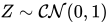
The standard complex normal random variable or standard complex Gaussian random variable is a complex random variable whose real and imaginary parts are independent normally distributed random variables with mean zero and variance .[3]:p. 494[4]:pp. 501 Formally,


where denotes independence and denotes that is a standard complex normal random variable.

Complex normal random variable
Suppose and are real random variables such that is a 2-dimensional normal random vector. Then the complex random variable is called complex normal random variable or complex Gaussian random variable.[3]:p. 500


Complex standard normal random vector
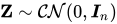
A n-dimensional complex random vector is a complex standard normal random vector or complex standard Gaussian random vector if its components are independent and all of them are standard complex normal random variables as defined above.[3]:p. 502[4]:pp. 501 That is a standard complex normal random vector is denoted .


Complex normal random vector
If and are random vectors in such that is a normal random vector with componentes. Entonces decimos que el vector aleatorio complejo



![{\displaystyle [\mathbf {X} ,\mathbf {Y} ]}](https://wikimedia.org/api/rest_v1/media/math/render/svg/39633a1d2cf0edd432b5ceee258360ac47ebf9db)


es un vector aleatorio normal complejo o un vector aleatorio gaussiano complejo .
Media, covarianza y relación
La distribución gaussiana compleja se puede describir con 3 parámetros: [ 5 ]
![{\displaystyle \mu =\operatorname {E} [\mathbf {Z} ],\quad \Gamma =\operatorname {E} [(\mathbf {Z} -\mu )({\mathbf {Z} }-\mu )^{\mathrm {H} }],\quad C=\operatorname {E} [(\mathbf {Z} -\mu )(\mathbf {Z} -\mu )^{\mathrm {T} }],}](https://wikimedia.org/api/rest_v1/media/math/render/svg/d8186b266f6fa5b1c962c01bcc77a666d4ae579b)
dóndedenota la transpuesta de la matriz de, ydenota transpuesta conjugada . [ 3 ] : pág. 504 [ 4 ] : págs. 500


Aquí el parámetro de ubicaciónes un vector complejo n-dimensional; la matriz de covarianzaes hermitiana y semidefinida positiva ; y, la matriz de relación o matriz de pseudocovarianzaes simétrico . El vector aleatorio normal complejoahora se puede denotar comoAdemás, matricesyson tales que la matriz



también es definida no negativa dondedenota el conjugado complejo de. [ 5 ]

Relaciones entre matrices de covarianza
Como ocurre con cualquier vector aleatorio complejo, las matricesypuede estar relacionado con las matrices de covarianza deya través de expresiones


![{\displaystyle {\begin{aligned}&V_{XX}\equiv \operatorname {E} [(\mathbf {X} -\mu _{X})(\mathbf {X} -\mu _{X})^{\mathrm {T} }]={\tfrac {1}{2}}\operatorname {Re} [\Gamma +C],\quad V_{XY}\equiv \operatorname {E} [(\mathbf {X} -\mu _{X})(\mathbf {Y} -\mu _{Y})^{\mathrm {T} }]={\tfrac {1}{2}}\operatorname {Im} [-\Gamma +C],\\&V_{YX}\equiv \operatorname {E} [(\mathbf {Y} -\mu _{Y})(\mathbf {X} -\mu _{X})^{\mathrm {T} }]={\tfrac {1}{2}}\operatorname {Im} [\Gamma +C],\quad \,V_{YY}\equiv \operatorname {E} [(\mathbf {Y} -\mu _ {Y})(\mathbf {Y} -\mu _{Y})^{\mathrm {T} }]={\tfrac {1}{2}}\operatorname {Re} [\Gamma -C],\end{alineado}}}](https://wikimedia.org/api/rest_v1/media/math/render/svg/7816194d319a6f156db69f13e9f2add16b9937fe)
y viceversa

Función de densidad
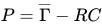
La función de densidad de probabilidad para la distribución normal compleja se puede calcular como
![{\displaystyle {\begin{aligned}f(z)&={\frac {1}{\pi ^{n}{\sqrt {\det(\Gamma )\det(P)}}}}\,\exp \!\left\{-{\frac {1}{2}}{\begin{bmatrix}z-\mu \\{\overline {z}}-{\overline {\mu }}\end{bmatrix}}^{\mathrm {H} }{\begin{bmatrix}\Gamma &C\\{\overline {C}}&{\overline {\Gamma }}\end{bmatrix}}^{\!\!-1}\!{\begin{bmatrix}z-\mu \\{\overline {z}}-{\overline {\mu }}\end{bmatrix}}\right\}\\[8pt]&={\tfrac {\sqrt {\det \left({\overline {P^{-1}}}-R^{\ast }P^{-1}R\right)\det(P^{-1})}}{\pi ^{n}}}\,e^{-(z-\mu )^{\ast }{\overline {P^{-1}}}(z-\mu )+\operatorname {Re} \left((z-\mu )^{\intercal }R^{\intercal }{\overline {P^{-1}}}(z-\mu )\right)},\end{aligned}}}](https://wikimedia.org/api/rest_v1/media/math/render/svg/736e45cbaf3e68d9ca78dbb9cafda0402ed3c4b3)
dóndey.

Función característica
La función característica de la distribución normal compleja viene dada por [ 5 ].

donde el argumentoes un vector complejo n -dimensional.

Propiedades
- Sies un vector normal complejo de n dimensiones,una matriz m×n , yun vector m constante , luego la transformación linealtambién se distribuirá de forma compleja-normal:



- Sies un vector normal complejo de n dimensiones , entonces
![{\displaystyle 2{\Big [}(\mathbf {Z} -\mu )^{\mathrm {H} }{\overline {P^{-1}}}(\mathbf {Z} -\mu )-\operatorname {Re} {\big (}(\mathbf {Z} -\mu )^{\mathrm {T} }R^{\mathrm {T} }{\overline {P^{-1}}}(\mathbf {Z} -\mu ){\big )}{\Big ]}\ \sim \ \chi ^{2}(2n)}](https://wikimedia.org/api/rest_v1/media/math/render/svg/a4752c39ed434c1a5f987accdda45de63384153f)
- Teorema del límite central . Sison variables aleatorias complejas independientes e idénticamente distribuidas, entonces

- dóndey.
![{\displaystyle {\sqrt {T}}{\Big (}{\tfrac {1}{T}}\textstyle \sum _{t=1}^{T}Z_{t}-\operatorname {E} [Z_{t}]{\Big )}\ \xrightarrow {d} \ {\mathcal {CN}}(0,\,\Gamma ,\,C),}](https://wikimedia.org/api/rest_v1/media/math/render/svg/7a8e03845ead334b995c22f8fb6a63887477b36d)
![{\displaystyle \Gamma =\operatorname {E} [ZZ^{\mathrm {H} }]}](https://wikimedia.org/api/rest_v1/media/math/render/svg/040fb5df40ce465da42594603d54e851879ccdf9)
![{\displaystyle C=\operatorname {E} [ZZ^{\mathrm {T} }]}](https://wikimedia.org/api/rest_v1/media/math/render/svg/d57ca27eba4a64bb77bac89459414af49a542522)
- El módulo de una variable aleatoria normal compleja sigue una distribución de Hoyt . [ 6 ]
Caso central de simetría circular
Definición
Un vector aleatorio complejose denomina simétrico circularmente si para cada deterministala distribución dees igual a la distribución de[ 4 ] : págs . 500–501


Los vectores aleatorios complejos normales centrales que son circularmente simétricos son de particular interés porque están completamente especificados por la matriz de covarianza..
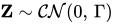
La distribución normal compleja circularmente simétrica (central) corresponde al caso de media cero y matriz de relación cero, es deciry. [ 3 ] : pág. 507 [ 7 ] Esto se suele denotar
Distribución de las partes real e imaginaria
Sies circularmente simétrico (central) normal complejo, entonces el vectores una distribución normal multivariada con estructura de covarianza


dónde.
![{\displaystyle \Gamma =\operatorname {E} [\mathbf {Z} \mathbf {Z} ^{\mathrm {H} }]}](https://wikimedia.org/api/rest_v1/media/math/render/svg/5664837bef03da1b45373e4aefa316892ccf80ed)
Función de densidad de probabilidad
Para una matriz de covarianza no singular, su distribución también puede simplificarse como [ 3 ] : pág. 508
- .

Por lo tanto, si la media no es ceroy matriz de covarianzason desconocidos, una función de verosimilitud logarítmica adecuada para un único vector de observaciónsería


La distribución normal compleja estándar (definida en la ecuación 1 ) corresponde a la distribución de una variable aleatoria escalar con,yPor lo tanto, la distribución normal compleja estándar tiene densidad

Propiedades
La expresión anterior demuestra por qué el caso,se denomina “circularmente simétrica”. La función de densidad depende únicamente de la magnitud depero no en su argumento . Como tal, la magnitudde una variable aleatoria normal compleja estándar tendrá la distribución de Rayleigh y la magnitud al cuadradotendrá la distribución exponencial , mientras que el argumento se distribuirá uniformemente en.


![{\displaystyle [-\pi ,\pi ]}](https://wikimedia.org/api/rest_v1/media/math/render/svg/cb064fd6c55820cfa660eabeeda0f6e3c4935ae6)
Sison vectores aleatorios normales complejos circulares n -dimensionales independientes e idénticamente distribuidos con, entonces la norma cuadrática aleatoria
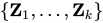
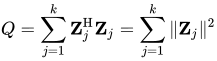
tiene la distribución chi-cuadrado generalizada y la matriz aleatoria
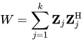
tiene la distribución compleja de Wishart congrados de libertad. Esta distribución se puede describir mediante la función de densidad.


dónde, yes unmatriz semidefinida positiva.


Véase también
- Distribución de razón normal compleja
- Estadísticas direccionales § Distribución de la media (forma polar)
- Distribución normal
- Distribución normal multivariada (una distribución normal compleja es una distribución normal bivariada)
- Distribución chi-cuadrado generalizada
- Distribución Wishart
- variable aleatoria compleja
Referencias
- ↑ Goodman, NR (1963). "Análisis estadístico basado en una cierta distribución gaussiana compleja multivariada (una introducción)" . The Annals of Mathematical Statistics . 34 (1): 152– 177. doi : 10.1214/aoms/1177704250 . JSTOR 2991290 .
- ↑ capítulo del libro, Gallager.R , pág. 9.
- 1 2 3 4 5 6 Lapidoth, A. (2009). Fundamentos de la comunicación digital . Cambridge University Press. ISBN 9780521193955.
- 1 2 3 4 Tse, David (2005). Fundamentos de la comunicación inalámbrica . Cambridge University Press. ISBN 9781139444668.
- 1 2 3 Picinbono, Bernard (1996). "Vectores aleatorios complejos de segundo orden y distribuciones normales" . IEEE Transactions on Signal Processing . 44 (10): 2637– 2640. Bibcode : 1996ITSP...44.2637P . doi : 10.1109/78.539051 .
- ↑ Daniel Wollschlaeger. "La distribución de Hoyt (Documentación para el paquete de R 'shotGroups' versión 0.6.2)" .
- ↑ capítulo del libro, Gallager.R
- Distribuciones continuas
- Distribuciones continuas multivariadas
- Distribuciones complejas