 Hispanopedia Wiki
In applied mathematics, the Joukowsky transform (sometimes transliterated Joukovsky, Joukowski or Zhukovsky) is a conformal map historically used to understand some principles of airfoil design. It is named after Nikolai Zhukovsky, who published it in 1910.[1]
The transform and its right-inverse are

where is a complex variable in the new space and is a complex variable in the original space. The right-inverse is not a global left-inverse because is 2-to-1; but a local left-inverse is always one of the right-inverse branches.


In aerodynamics, the transform is used to solve for the two-dimensional potential flow around a class of airfoils known as Joukowsky airfoils. A Joukowsky airfoil is generated in the complex plane (-plane) by applying the Joukowsky transform to a circle in the -plane. The coordinates of the centre of the circle are variables, and varying them modifies the shape of the resulting airfoil. The circle encloses the point (where the derivative is zero) and intersects the point This can be achieved for any allowable centre position by varying the radius of the circle.


Joukowsky airfoils have a cusp at their trailing edge. A closely related conformal mapping, the Kármán–Trefftz transform, generates the broader class of Kármán–Trefftz airfoils by controlling the trailing edge angle. When a trailing edge angle of zero is specified, the Kármán–Trefftz transform reduces to the Joukowsky transform.
General Joukowsky transform
The Joukowsky transform of any complex number to is as follows:
![{\displaystyle {\begin{aligned}z&=x+iy=\zeta +{\frac {1}{\zeta }}\\&=\chi +i\eta +{\frac {1}{\chi +i\eta }}\\[2pt]&=\chi +i\eta +{\frac {\chi -i\eta }{\chi ^{2}+\eta ^{2}}}\\[2pt]&=\chi \left(1+{\frac {1}{\chi ^{2}+\eta ^{2}}}\right)+i\eta \left(1-{\frac {1}{\chi ^{2}+\eta ^{2}}}\right).\end{aligned}}}](https://wikimedia.org/api/rest_v1/media/math/render/svg/8e2b2f8c9848f1657d05a4cc14dd96c9a3e87507)
So the real () and imaginary () components are:


![{\displaystyle {\begin{aligned}x&=\chi \left(1+{\frac {1}{\chi ^{2}+\eta ^{2}}}\right),\\[2pt]y&=\eta \left(1-{\frac {1}{\chi ^{2}+\eta ^{2}}}\right).\end{aligned}}}](https://wikimedia.org/api/rest_v1/media/math/render/svg/f0a50c5ba8c65bcd954c518839f845f2acb3e598)
Sample Joukowsky airfoil
The transformation of all complex numbers on the unit circle is a special case.
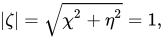
which gives
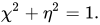
So the real component becomes and the imaginary component becomes .


Thus the complex unit circle maps to a flat plate on the real-number line from −2 to +2.
Transformations from other circles make a wide range of airfoil shapes.
Velocity field and circulation for the Joukowsky airfoil
The solution to potential flow around a circular cylinder is analytic and well known. It is the superposition of uniform flow, a doublet, and a vortex.
The complex conjugate velocity around the circle in the -plane is
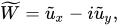

where
- is the complex coordinate of the centre of the circle,
- is the freestream velocity of the fluid,
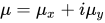

is the angle of attack of the airfoil with respect to the freestream flow,

- is the radius of the circle, calculated using ,
- is the circulation, found using the Kutta condition, which reduces in this case to

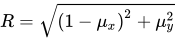


The complex velocity around the airfoil in the -plane is, according to the rules of conformal mapping and using the Joukowsky transformation,


Here with and the velocity components in the and directions respectively ( with and real-valued). From this velocity, other properties of interest of the flow, such as the coefficient of pressure and lift per unit of span can be calculated.



Kármán–Trefftz transform


The Kármán–Trefftz transform is a conformal map closely related to the Joukowsky transform. While a Joukowsky airfoil has a cusped trailing edge, a Kármán–Trefftz airfoil—which is the result of the transform of a circle in the -plane to the physical -plane, analogue to the definition of the Joukowsky airfoil—has a non-zero angle at the trailing edge, between the upper and lower airfoil surface. The Kármán–Trefftz transform therefore requires an additional parameter: the trailing-edge angle This transform is[2][3]

where is a real constant that determines the positions where , and is slightly smaller than 2. The angle between the tangents of the upper and lower airfoil surfaces at the trailing edge is related to as[2]



The derivative , required to compute the velocity field, is

![{\displaystyle {\frac {dz}{d\zeta }}={\frac {4n^{2}}{\zeta ^{2}-1}}{\frac {\left(1+{\frac {1}{\zeta }}\right)^{n}\left(1-{\frac {1}{\zeta }}\right)^{n}}{\left[\left(1+{\frac {1}{\zeta }}\right)^{n}-\left(1-{\frac {1}{\zeta }}\right)^{n}\right]^{2}}}.}](https://wikimedia.org/api/rest_v1/media/math/render/svg/9e8c37052334854a67b3388bf8047e96fbc966a3)
Background
First, add and subtract 2 from the Joukowsky transform, as given above:
![{\displaystyle {\begin{aligned}z+2&=\zeta +2+{\frac {1}{\zeta }}={\frac {1}{\zeta }}(\zeta +1)^{2},\\[3pt]z-2&=\zeta -2+{\frac {1}{\zeta }}={\frac {1}{\zeta }}(\zeta -1)^{2}.\end{aligned}}}](https://wikimedia.org/api/rest_v1/media/math/render/svg/ef1652730dc32a9ba2669f06a26a1aa45cb43455)
Dividing the left and right hand sides gives
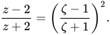
The right hand side contains (as a factor) the simple second-power law from potential flow theory, applied at the trailing edge near From conformal mapping theory, this quadratic map is known to change a half plane in the -space into potential flow around a semi-infinite straight line. Further, values of the power less than 2 will result in flow around a finite angle. So, by changing the power in the Joukowsky transform to a value slightly less than 2, the result is a finite angle instead of a cusp. Replacing 2 by in the previous equation gives[2]

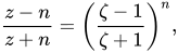
which is the Kármán–Trefftz transform. Solving for gives it in the form of equation A.
Symmetrical Joukowsky airfoils
In 1943 Hsue-shen Tsien published a transform of a circle of radius into a symmetrical airfoil that depends on parameter and angle of inclination :[4]



The parameter yields a flat plate when zero, and a circle when infinite; thus it corresponds to the thickness of the airfoil. Furthermore the radius of the cylinder .

Notes
- ↑Joukowsky, N. E. (1910). "Über die Konturen der Tragflächen der Drachenflieger". Zeitschrift für Flugtechnik und Motorluftschiffahrt (in German). 1: 281–284 and (1912) 3: 81–86.
- 123Milne-Thomson, Louis M. (1973). Theoretical aerodynamics (4th ed.). Dover Publ. pp. 128–131. ISBN 0-486-61980-X.
- ↑Blom, J. J. H. (1981). "Some Characteristic Quantities of Karman-Trefftz Profiles" (Document). NASA Technical Memorandum TM-77013.
- ↑Tsien, Hsue-shen (1943). "Symmetrical Joukowsky airfoils in shear flow". Quarterly of Applied Mathematics. 1 (2): 130–248. doi:10.1090/qam/8537.
References
External links
- Joukowski Transform NASA Applet
- Joukowsky Transform Interactive WebApp
- Conformal mappings
- Aircraft aerodynamics
- Aircraft wing design