 Hispanopedia Wiki
En matemáticas , una cuádrica o superficie cuádrica es una generalización de las secciones cónicas ( elipses , parábolas e hipérbolas ). En el espacio tridimensional , las cuádricas incluyen elipsoides , paraboloides e hiperboloides .
De forma más general, una hipersuperficie cuádrica (de dimensión D ) incrustada en un espacio de dimensión superior (de dimensión D + 1 ) se define como el conjunto cero de un polinomio irreducible de grado dos en D + 1 variables; por ejemplo, D = 1 es el caso de las secciones cónicas ( curvas planas ). Cuando el polinomio definitorio no es absolutamente irreducible , el conjunto cero generalmente no se considera una cuádrica, aunque a menudo se le llama cuádrica degenerada o cuádrica reducible .
Una cuádrica es una variedad algebraica afín o, si es reducible, un conjunto algebraico afín . Las cuádricas también pueden definirse en espacios proyectivos ; véase la sección « Forma normal de las cuádricas proyectivas» , más adelante.
Formulación
En coordenadas x 1 , x 2 , ..., x D +1 , la cuádrica general se define así por la ecuación algebraica [ 1 ].
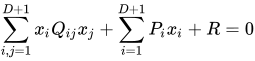
que se puede escribir de forma compacta en notación vectorial y matricial como:

donde x = ( x 1 , x 2 , ..., x D +1 ) es un vector fila , x T es la transpuesta de x (un vector columna ), Q es una matriz ( D + 1) × ( D + 1) y P es un vector fila de dimensión ( D + 1) y R una constante escalar. Los valores Q , P y R a menudo se toman sobre números reales o números complejos , pero una cuádrica puede definirse sobre cualquier cuerpo .
plano euclidiano
Las cuádricas en un plano euclidiano tienen dimensión uno y, por lo tanto, son curvas planas . Se denominan secciones cónicas o cónicas .

espacio euclidiano
En el espacio euclidiano tridimensional , las cuádricas tienen dimensión dos y se conocen como superficies cuádricas . Sus ecuaciones cuadráticas tienen la formaodóndey


Las superficies cuádricas se clasifican y nombran según su forma, que corresponde a las órbitas bajo transformaciones afines . Es decir, si una transformación afín transforma una superficie cuádrica en otra, pertenecen a la misma clase y comparten el mismo nombre y muchas propiedades.
El teorema de los ejes principales demuestra que, para cualquier cuádrica (posiblemente reducible), un cambio adecuado de coordenadas cartesianas o, equivalentemente, una transformación euclidiana permite expresar la ecuación de la cuádrica en una forma simple única en la que la clase de la cuádrica es inmediatamente visible. Esta forma se denomina forma normal de la ecuación, ya que dos cuádricas tienen la misma forma normal si y solo si existe una transformación euclidiana que mapea una cuádrica en la otra. Las formas normales son las siguientes:

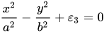
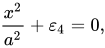
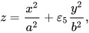
donde elson 1, −1 o 0, exceptoque solo toma el valor 0 o 1.


Cada una de estas 17 formas normales [ 2 ] corresponde a una sola órbita bajo transformaciones afines. En tres casos no hay puntos reales:( elipsoide imaginario ),( cilindro elíptico imaginario ), y(par de planos paralelos conjugados complejos , una cuádrica reducible). En un caso, el cono imaginario , hay un único punto (). Siuno tiene una línea (de hecho, dos planos complejos conjugados que se intersecan). Parauno tiene dos planos que se intersecan (cuádrica reducible). Parauno tiene un plano doble. Parauna tiene dos planos paralelos (cuádrica reducible).






Así, entre las 17 formas normales, hay nueve cuádricas verdaderas: un cono, tres cilindros (a menudo llamados cuádricas degeneradas) y cinco cuádricas no degeneradas ( elipsoide , paraboloides e hiperboloides ), que se detallan en las siguientes tablas. Las ocho cuádricas restantes son el elipsoide imaginario (sin punto real), el cilindro imaginario (sin punto real), el cono imaginario (con un único punto real) y las cuádricas reducibles, que se descomponen en dos planos; existen cinco de estas cuádricas descompuestas, dependiendo de si los planos son distintos o no, paralelos o no, reales o complejos conjugados.
Cuando dos o más de los parámetros de la ecuación canónica son iguales, se obtiene una cuádrica de revolución , que permanece invariante al girar alrededor de un eje (o infinitos ejes, en el caso de la esfera).
Intersección de un rayo con una superficie cuádrica
Fuente: [ 3 ]
Se puede representar un rayo tridimensional paramétricamente como dónde,, yson los,, ycomponentes del vector de dirección normalizado del rayo yes la distancia a lo largo del rayo. Insertando estos valores en la ecuación para una superficie cuádrica tridimensional, se obtiene una ecuación cuadrática paraSi existen dos raíces reales, esto proporciona los dos puntos de intersección del rayo con la superficie cuádrica. Si existe una raíz doble, el rayo roza la superficie. Si no existen raíces reales, el rayo no alcanza la superficie cuádrica.


Alternativamente, utilizando coordenadas homogéneas , se puede representar el rayo como [ 4 ] [ 5 ]dóndees una línea que pasa por el puntoyes el vector de dirección del rayo. La ecuación para la intersección de un rayo con una superficie cuádrica se representa entonces comolo que produce la misma ecuación cuadrática en t .


La normal a cualquier punto de la superficie es

Parches de superficie cuádricos en el trazado de rayos gráfico
En gráficos por computadora, la representación visual de objetos modelados matemáticamente se determina frecuentemente mediante trazado de rayos . A menudo, las superficies de los objetos se describen en términos de una serie de puntos en la superficie y las normales a la superficie en esos puntos. Los puntos intermedios en la superficie se describen mediante un conjunto de parches de superficie entre los puntos. Las superficies cuádricas se utilizan frecuentemente de esta manera cuando la superficie se describe como un conjunto de triángulos utilizando las posiciones y normales a los vértices de esos triángulos. El uso de superficies cuádricas para modelar estos parches tiene la ventaja de que es fácil determinar si un rayo de luz interseca un parche y dónde lo hace, como se describió en la sección anterior. [ 4 ] [ 5 ]
La ecuación para una superficie cuádrica tiene diez variables, pero solo nueve variables independientes, ya que la multiplicación de la ecuación por cualquier constante distinta de cero no tiene efecto. Las normales y las ubicaciones de tres puntos dan nueve restricciones. Por lo tanto, parecería posible determinar de forma única un parche triangular de superficie cuádrica a partir de esta información. De hecho, se puede construir unamatriz lineal para designar estas restricciones. Sin embargo, se puede demostrar que esta matriz siempre será singular, por lo que se debe agregar alguna restricción adicional para determinar de manera única la superficie cuádrica de ese parche. [ 6 ]

Determinación del tipo de superficie cuádrica y el desplazamiento desde la posición estándar.
Fuentes: [ 7 ] [ 8 ]
En general, las ecuaciones cuádricas pueden no estar en forma normal, y puede ser difícil determinar el tipo de superficie cuádrica mediante inspección visual a menos que la superficie cuádrica tenga su centro en el origen y los ejes principales estén a lo largo de las direcciones x , y y z. Sin embargo, si se define la submatriz deLuego, la siguiente tabla permite clasificar la superficie cuádrica, basándose en los rangos , determinantes y valores propios de laymatrices.


Todas las superficies cuádricas reales, excepto los elipsoides y los hiperboloides, son casos límite especiales. Cualquier elipsoide o hiperboloides real se puede expresar como una matriz reposicionada de la formaconque contiene únicamente los componentes diagonales de, y, siendo los demás ceros. Aquí las columnas de los ejes x , y y z de la matriz afínson los autovectores normalizados de. donde el acento agudo implica la transpuesta de la matriz. La ubicación del centroide ,(en la cuarta columna de) esLos radios de los ejes tienen los valoresdonde los ejes radiales y a lo largo de los autovectores de los autovalores correspondientes, yPara un elipsoide real, los radios de todos los autovalores son positivos. Para un hiperboloide de una hoja, uno de los radios al cuadrado es negativo, siendo los otros dos los de la elipse en el cuello del hiperboloide. Para un hiperboloide de dos hojas, dos de los radios al cuadrado son negativos y el radio real es la distancia desde el centro hasta los vértices de las hojas. Si los tres autovalores dan radios al cuadrado negativos, entonces la superficie cuádrica es un elipsoide imaginario. [ 7 ]


Transformación afín de superficie cuádrica
Las matrices de transformación afín se utilizan para representar transformaciones de coordenadas. Dicha matriz tiene la forma [ 9 ] [ 10 ].Aquí la primera columna de la matriz es el vector de dirección normalizado de la-eje del nuevo sistema de coordenadas, con respecto al sistema de coordenadas original,La segunda columna representa laeje -, la tercera columna-eje, y la cuarta columna es la ubicación del origen enen el sistema de coordenadas original. Un punto en la ubicación, en términos de laEl sistema de coordenadas está en el puntoen el sistema de coordenadas original. Tenga en cuenta que aquí, elEl vector tiene un "1" como su cuarto término, ya que es un vector de ubicación, mientras que los vectores de dirección tienen un "0" como cuarto término. Usando las reglas habituales del álgebra matricial, la transformación inversa se obtiene como la inversa de la matriz., eso es,Estas transformaciones se pueden concatenar, de modo que si hay un sistema de coordenadas, con una ubicación y orientacióncon respecto a, su orientación con respecto aescomo se calcula mediante multiplicación de matrices. Estas matrices de transformación se utilizan frecuentemente para calcular las ubicaciones y la orientación de los vehículos. Por ejemplo, una aeronave en un puntoen el marco de referencia de la aeronave estará en un puntoen el sistema de coordenadas terrestres, sies la transformación entre el sistema de referencia terrestre y el sistema de referencia de la aeronave.


Las superficies cuádricas tienen la agradable propiedad de que también se transforman bajo transformaciones de coordenadas afines. Si una superficie cuádrica,, is moved to a coordinate location and orientation , its description as seen from the original coordinate system is[11]However, this needs to be distinguished from a quadric surface defined in coordinate system as viewed from a coordinate system , where the transformation is


Note that since , it does not matter whether or not this matrix is transposed, and one may see it either way in the literature.

Latitude, longitude, and altitude as quadric surfaces
Latitude and longitude are normally thought of as lines on the globe, but when you consider that one may cross a line of latitude or longitude at different altitudes, it becomes obvious that these lines are actually surfaces, in fact, quadric surfaces. If the Earth is approximated as a sphere, longitudes are planes slicing though the center of the Earth and through the poles, while latitudes are cones, with the point of the cone at the center of the Earth. Altitudes are spheres of different radii. This is the general model currently used for naval and aviation navigation.
When the Earth is better approximated as an ellipsoid, the longitudes are still the same planes as for the spherical Earth. Latitudes are still cones, but the points of the cones are no longer at the center of the Earth, except at the equator; the cone axis is still along the Earth's axis, but north or south of the Earth center. Altitudes are ellipsoids. In the World Geodetic System 1984 (WGS84), the equatorial radius of the Earth is () is given as 6,378,137.0 meters and the polar radius () as 6,356,752.3142 meters. The squared first eccentricity is then


Given latitude and longitude , Earth-centered (geocentric) coordinates can be determined as[12] where H is the height above the Earth ellipsoid and


Definition and basic properties
An affine quadric is the set of zeros of a polynomial of degree two. When not specified otherwise, the polynomial is supposed to have real coefficients, and the zeros are points in a Euclidean space. However, most properties remain true when the coefficients belong to any field and the points belong in an affine space. As usual in algebraic geometry, it is often useful to consider points over an algebraically closed field containing the polynomial coefficients, generally the complex numbers, when the coefficients are real.
Muchas propiedades se vuelven más fáciles de enunciar (y de demostrar) extendiendo la cuádrica al espacio proyectivo mediante la completación proyectiva , que consiste en agregar puntos en el infinito . Técnicamente, si
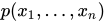
es un polinomio de grado dos que define una cuádrica afín, entonces su completación proyectiva se define homogeneizando p en

( esto es un polinomio, porque el grado de p es dos). Los puntos de la completación proyectiva son los puntos del espacio proyectivo cuyas coordenadas proyectivas son ceros de P.
Así pues, una cuádrica proyectiva es el conjunto de ceros en un espacio proyectivo de un polinomio homogéneo de grado dos.
Como el proceso de homogeneización anterior se puede revertir estableciendo X 0 = 1 :

A menudo resulta útil no distinguir una cuádrica afín de su completación proyectiva, y hablar de la ecuación afín o la ecuación proyectiva de una cuádrica. Sin embargo, esto no es una equivalencia perfecta; generalmente sucede queincluirá puntos con, que no son también soluciones deporque estos puntos en el espacio proyectivo corresponden a puntos "en el infinito" en el espacio afín.


Ecuación
Una cuádrica en un espacio afín de dimensión n es el conjunto de ceros de un polinomio de grado 2. Es decir, es el conjunto de los puntos cuyas coordenadas satisfacen una ecuación

donde el polinomio p tiene la forma

para una matrizconycorriendo de 0 aCuando la característica del campo de los coeficientes no es dos, generalmentese supone; equivalentementeCuando la característica del campo de los coeficientes es dos, generalmentese asume cuando; equivalentementees triangular superior .


La ecuación puede acortarse, como la ecuación matricial.

con

La ecuación de la completación proyectiva es casi idéntica:

con

Estas ecuaciones definen una cuádrica como una hipersuperficie algebraica de dimensión n − 1 y grado dos en un espacio de dimensión n .
Se dice que una cuádrica no es degenerada si la matrizes invertible .
Una cuádrica no degenerada es no singular en el sentido de que su completación proyectiva no tiene un punto singular (un cilindro es no singular en el espacio afín, pero es una cuádrica degenerada que tiene un punto singular en el infinito ).
The singular points of a degenerate quadric are the points whose projective coordinates belong to the null space of the matrix A.
A quadric is reducible if and only if the rank of A is one (case of a double hyperplane) or two (case of two hyperplanes).
Normal form of projective quadrics
In real projective space, by Sylvester's law of inertia, a non-singular quadratic formP(X) may be put into the normal form

by means of a suitable projective transformation (normal forms for singular quadrics can have zeros as well as ±1 as coefficients). For two-dimensional surfaces (dimension D = 2) in three-dimensional space, there are exactly three non-degenerate cases:
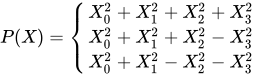
The first case is the empty set.
The second case generates the ellipsoid, the elliptic paraboloid or the hyperboloid of two sheets, depending on whether the chosen plane at infinity cuts the quadric in the empty set, in a point, or in a nondegenerate conic respectively. These all have positive Gaussian curvature.
The third case generates the hyperbolic paraboloid or the hyperboloid of one sheet, depending on whether the plane at infinity cuts it in two lines, or in a nondegenerate conic respectively. These are doubly ruled surfaces of negative Gaussian curvature.
The degenerate form

generates the elliptic cylinder, the parabolic cylinder, the hyperbolic cylinder, or the cone, depending on whether the plane at infinity cuts it in a point, a line, two lines, or a nondegenerate conic respectively. These are singly ruled surfaces of zero Gaussian curvature.
We see that projective transformations don't mix Gaussian curvatures of different sign. This is true for general surfaces.[13]
In complex projective space all of the nondegenerate quadrics become indistinguishable from each other.
Rational parametrization
Dado un punto no singular A de una cuádrica, una línea que pasa por A es tangente a la cuádrica o la interseca en exactamente otro punto (como es habitual, una línea contenida en la cuádrica se considera tangente, puesto que está contenida en el hiperplano tangente ). Esto significa que las líneas que pasan por A y no son tangentes a la cuádrica están en correspondencia biunívoca con los puntos de la cuádrica que no pertenecen al hiperplano tangente en A. Expresar los puntos de la cuádrica en términos de la dirección de la línea correspondiente proporciona ecuaciones paramétricas de las siguientes formas.
En el caso de secciones cónicas (curvas cuádricas), esta parametrización establece una biyección entre una sección cónica proyectiva y una recta proyectiva ; esta biyección es un isomorfismo de curvas algebraicas . En dimensiones superiores, la parametrización define una aplicación birracional , que es una biyección entre subconjuntos abiertos densos de la cuádrica y un espacio proyectivo de la misma dimensión (la topología que se considera es la usual en el caso de una cuádrica real o compleja, o la topología de Zariski en todos los casos). Los puntos de la cuádrica que no están en la imagen de esta biyección son los puntos de intersección de la cuádrica y su hiperplano tangente en A.
En el caso afín, la parametrización es una parametrización racional de la forma

dóndeson las coordenadas de un punto de la cuádrica,son parámetros yson polinomios de grado como máximo dos.


En el caso proyectivo, la parametrización tiene la forma

dóndeson las coordenadas proyectivas de un punto de la cuádrica,son parámetros yson polinomios homogéneos de grado dos.


Se pasa de una parametrización a la otra colocandoy
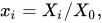


Para calcular la parametrización y demostrar que los grados son los afirmados, se puede proceder de la siguiente manera en el caso afín. En el caso proyectivo, se puede proceder de forma similar.
Sea q el polinomio cuadrático que define la cuádrica, ysea el vector de coordenadas del punto dado de la cuádrica (entonces,Dejarsea el vector de coordenadas del punto de la cuádrica que se va a parametrizar, ysea un vector que defina la dirección utilizada para la parametrización (las direcciones cuya última coordenada es cero no se tienen en cuenta aquí; esto significa que algunos puntos de la cuádrica afín no están parametrizados; a menudo se dice que están parametrizados por puntos en el infinito en el espacio de parámetros). Los puntos de intersección de la cuádrica y la línea de dirección passing through are the points such that






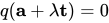
for some value of the scalar This is an equation of degree two in except for the values of such that the line is tangent to the quadric (in this case, the degree is one if the line is not included in the quadric, or the equation becomes otherwise). The coefficients of and are respectively of degree at most one and two in As the constant coefficient is the equation becomes linear by dividing by and its unique solution is the quotient of a polynomial of degree at most one by a polynomial of degree at most two. Substituting this solution into the expression of one obtains the desired parametrization as fractions of polynomials of degree at most two.


Example: circle and spheres
Let consider the quadric of equation

For this is the unit circle; for this is the unit sphere; in higher dimensions, this is the unit hypersphere.


The point belongs to the quadric (the choice of this point among other similar points is only a question of convenience). So, the equation of the preceding section becomes


By expanding the squares, simplifying the constant terms, dividing by and solving in one obtains
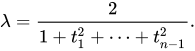
Substituting this into and simplifying the expression of the last coordinate, one obtains the parametric equation
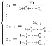
By homogenizing, one obtains the projective parametrization
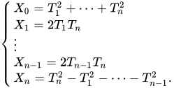
A straightforward verification shows that this induces a bijection between the points of the quadric such that and the points such that in the projective space of the parameters. On the other hand, all values of such that and give the point




In the case of conic sections (), there is exactly one point with and one has a bijection between the circle and the projective line.


For there are many points with and thus many parameter values for the point On the other hand, the other points of the quadric for which (and thus ) cannot be obtained for any value of the parameters. These points are the points of the intersection of the quadric and its tangent plane at In this specific case, these points have nonreal complex coordinates, but it suffices to change one sign in the equation of the quadric for producing real points that are not obtained with the resulting parametrization.


Rational points
A quadric is defined over a field if the coefficients of its equation belong to When is the field of the rational numbers, one can suppose that the coefficients are integers by clearing denominators.


A point of a quadric defined over a field is said rational over if its coordinates belong to . A rational point over the field of the real numbers is called a real point.

A rational point over is called simply a rational point. By clearing denominators, one can suppose and one supposes generally that the projective coordinates of a rational point (in a quadric defined over ) are integers. Also, by clearing denominators of the coefficients, one supposes generally that all the coefficients of the equation of the quadric and the polynomials occurring in the parametrization are integers.
Finding the rational points of a projective quadric amounts thus to solving a Diophantine equation.
Given a rational point A over a quadric over a field F, the parametrization described in the preceding section provides rational points when the parameters are in F, and, conversely, every rational point of the quadric can be obtained from parameters in F, if the point is not in the tangent hyperplane at A.
It follows that, if a quadric has a rational point, it has many other rational points (infinitely many if F is infinite), and these points can be algorithmically generated as soon one knows one of them.
As said above, in the case of projective quadrics defined over the parametrization takes the form

where the are homogeneous polynomials of degree two with integer coefficients. Because of the homogeneity, one can consider only parameters that are setwise coprime integers. If is the equation of the quadric, a solution of this equation is said primitive if its components are setwise coprime integers. The primitive solutions are in one to one correspondence with the rational points of the quadric (up to a change of sign of all components of the solution). The non-primitive integer solutions are obtained by multiplying primitive solutions by arbitrary integers; so they do not deserve a specific study. However, setwise coprime parameters can produce non-primitive solutions, and one may have to divide by a greatest common divisor to arrive at the associated primitive solution.


Pythagorean triples
This is well illustrated by Pythagorean triples. A Pythagorean triple is a triple of positive integers such that A Pythagorean triple is primitive if are setwise coprime, or, equivalently, if any of the three pairs and is coprime.


By choosing and , the above method provides the parametrization


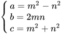
for the quadric of equation (The names of variables and parameters are being changed from the above ones to those that are common when considering Pythagorean triples).

If m and n are coprime integers such that La terna resultante es una terna pitagórica. Si uno de los términos m y n es par y el otro impar, esta terna resultante es primitiva; de lo contrario, ambos m y n son impares, y se obtiene una terna primitiva dividiendo por 2.

En resumen, las ternas pitagóricas primitivas conincluso se obtienen como


con m y n enteros coprimos tales que uno es par y(esta es la fórmula de Euclides ). Las ternas pitagóricas primitivas conLos impares se obtienen como


con m y n enteros impares coprimos tales que

Como el intercambio de a y b transforma una terna pitagórica en otra terna pitagórica, solo uno de los dos casos es suficiente para producir todas las ternas pitagóricas primitivas hasta el orden de a y b .
Cuádricas proyectivas sobre campos
La definición de una cuádrica proyectiva en un espacio proyectivo real (véase más arriba) puede adaptarse formalmente definiendo una cuádrica proyectiva en un espacio proyectivo n -dimensional sobre un cuerpo . Para evitar el uso de coordenadas, una cuádrica proyectiva se define generalmente partiendo de una forma cuadrática en un espacio vectorial. [ 14 ]
Forma cuadrática
Dejarser un campo yun espacio vectorial sobreUn mapeodeade tal manera que


- (P1)para cualquiery.



- (P2)es una forma bilineal .

Se denomina forma cuadrática . La forma bilineal.es simétrico .

En caso deLa forma bilineal es, es deciryse determinan mutuamente de una manera única. En caso de(eso significa:) la forma bilineal tiene la propiedad, es decires simpléctico .




Paray (es una base de)tiene la forma familiar

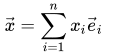


- y
- .

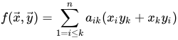
Por ejemplo:

espacio proyectivo n -dimensional sobre un campo
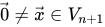
Dejarser un campo,,

- un espacio vectorial de ( n + 1) dimensiones sobre el campo
- el subespacio unidimensional generado por,
- el conjunto de puntos ,
- el conjunto de líneas .
- es el espacio proyectivo n -dimensional sobre.
- El conjunto de puntos contenidos en unsubespacio -dimensional dees unsubespacio -dimensional de. Un subespacio bidimensional es un plano .
- En caso deaEl subespacio de -dimensiones se llama hiperplano .







cuádrica proyectiva
Una forma cuadrática on a vector space defines a quadric in the associated projective space as the set of the points such that . That is,



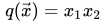
Examples in .:(E1): For one obtains a conic. (E2): For one obtains the pair of lines with the equations and , respectively. They intersect at point ;




For the considerations below it is assumed that .

Polar space
For point the set
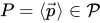

is called polar space of (with respect to ).

If for all , one obtains .


If for at least one , the equation is a non trivial linear equation which defines a hyperplane. Hence

- is either a hyperplane or .


Intersection with a line
For the intersection of an arbitrary line with a real quadric , the following cases may occur:

- a) and is called exterior line
- b) and is called a line in the quadric
- c) and is called tangent line
- d) and is called secant line.


Proof: Let be a line, which intersects at point and is a second point on . From one obtains I) In case of the equation holds and it is for any . Hence either for any or for any, which proves b) and b'). II) In case of one obtains and the equation has exactly one solution . Hence: , which proves c).













Additionally the proof shows:
- A line through a point is a tangent line if and only if .


f-radical, q-radical
In the classical cases or there exists only one radical, because of and and are closely connected. In case of the quadric is not determined by (see above) and so one has to deal with two radicals:


- a) is a projective subspace. is called f-radical of quadric .
- b) is called singular radical or -radical of .
- c) In case of one has .



A quadric is called non-degenerate if .

Examples in (see above): (E1): For (conic) the bilinear form is In case of the polar spaces are never . Hence . In case of the bilinear form is reduced to and . Hence In this case the f-radical is the common point of all tangents, the so called knot. In both cases and the quadric (conic) ist non-degenerate. (E2): For (pair of lines) the bilinear form is and the intersection point. In this example the quadric is degenerate.







Symmetries
A quadric is a rather homogeneous object:
- For any point there exists an involutorial central collineation with center and .


Proof: Due to the polar space is a hyperplane.

The linear mapping
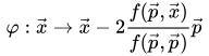
- :{\vec {x}}\rightarrow {\vec {x}}-{\frac {f({\vec {p}},{\vec {x}})}{q({\vec {p}})}}{\vec {p}}}
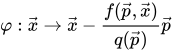
induces an involutorial central collineation with axis and centre which leaves invariant. In the case of , the mapping produces the familiar shape :{\vec {x}}\rightarrow {\vec {x}}-2{\frac {f({\vec {p}},{\vec {x}})}{f({\vec {p}},{\vec {p}})}}{\vec {p}}\;} with and for any .



Remark:
- a) An exterior line, a tangent line or a secant line is mapped by the involution on an exterior, tangent and secant line, respectively.
- b) is pointwise fixed by .
q-subspaces and index of a quadric
A subspace of is called -subspace if


For example: points on a sphere or lines on a hyperboloid (s. below).
- Any two maximal-subspaces have the same dimension .[15]

Let be the dimension of the maximal -subspaces of then
- The integer is called index of .

Theorem:[16]
- For the index of a non-degenerate quadric in the following is true:
- .

Let be a non-degenerate quadric in , and its index.
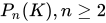
- In case of quadric is called sphere (or oval conic if ).
- In case of quadric is called hyperboloid (of one sheet).


Examples:
- a) Quadric in with form is non-degenerate with index 1.
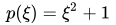
- b) If polynomial is irreducible over the quadratic form gives rise to a non-degenerate quadric in of index 1 (sphere). For example: is irreducible over (but not over !).
- c) In the quadratic form generates a hyperboloid.




Generalization of quadrics: quadratic sets
It is not reasonable to formally extend the definition of quadrics to spaces over genuine skew fields (division rings). Because one would obtain secants bearing more than 2 points of the quadric which is totally different from usual quadrics.[17][18][19] The reason is the following statement.
- A division ring is commutative if and only if any equation, has at most two solutions.

There are generalizations of quadrics: quadratic sets.[20] A quadratic set is a set of points of a projective space with the same geometric properties as a quadric: every line intersects a quadratic set in at most two points or is contained in the set.
See also
Referencias
- ↑ Silvio Levy, Cuadráticas en "Fórmulas y hechos de geometría", extracto de la 30.ª edición de Tablas y fórmulas matemáticas estándar de CRC , CRC Press , del Centro de Geometría de la Universidad de Minnesota.
- ↑ Stewart Venit y Wayne Bishop, Álgebra lineal elemental (cuarta edición) , International Thompson Publishing, 1996.
- ↑ Owen, Scott (7 de diciembre de 2025). "Intersección de rayos y cuádricas" .
{{cite web}}: CS1 mantenimiento: estado de la URL ( enlace ) - 1 2 Lawlor, Orion (3 de diciembre de 2025). "Intersección rayo-objeto para planos, esferas y cuádricas" . Archivado del original el 2 de julio de 2023.
- 1 2 House, Donald (4 de diciembre de 2025). "Sistemas de coordenadas" (PDF) . Archivado (PDF) del original el 6 de mayo de 2025.
- ↑ Birdal, Talga; Busam, Benjamin; Navab, Nassir; Ilic, Slobodan; Sturm, Peter (4 de enero de 2019). "Detección genérica de primitivas en nubes de puntos mediante ajustes cuadráticos mínimos novedosos" (PDF) . IEEE Transactions on Pattern Analysis and Machine Intelligence . 42 (6): 1333– 1347 – vía HAL.
- 1 2 Olmsted, John (marzo de 1945). "Matrices y superficies cuádricas" . National Mathematics Magazine . 19 (6): 267– 275 – vía Taylor & Francis.
- ↑ Olmsted, John (1 de enero de 1947). Geometría analítica sólida . D. Appleton-Century Company Inc. pp. Capítulo V. ASIN B0006AR5WU .
- ↑ "Matriz de transformación" , Wikipedia , 16 de julio de 2025 , consultado el 4 de diciembre de 2025.
- ↑ Kuipers, Jack (14 de diciembre de 1998). Cuaterniones y secuencias de rotación . Princeton University Press (publicado en 1999). págs. Capítulo 3: Rotaciones en el espacio tridimensional. ISBN 978-0691058726.
- ↑ House, Donald (4 de diciembre de 2025). "Superficies cuádricas" (PDF) . Archivado (PDF) del original el 1 de mayo de 2025.
- ↑ Toms, Ralph (11–15 de marzo de 1006). "Un algoritmo mejorado para la conversión de coordenadas geocéntricas a geodésicas" . Decimocuarto taller sobre estándares para simulaciones interactivas distribuidas, Orlando, Florida .
- ↑ S. Lazebnik y J. Ponce, "La forma proyectiva local de superficies lisas y sus contornos" (PDF) ., Proposición 1
- ↑ Beutelspacher/Rosenbaum p.158
- ↑ Beutelpacher/Rosenbaum, p.139
- ↑ F. Buekenhout: Ensembles Quadratiques des Espace Projective , Matemáticas. Teitschr. 110 (1969), pág. 306-318.
- ↑ R. Artzy : La Cónicaen Moufang Planes , Aequat.Mathem. 6 (1971), pág. 31-35
- ↑ E. Berz: Kegelschnitte en Desarguesschen Ebenen , Matemáticas. Zeitschr. 78 (1962), pág. 55-8
- ↑ enlace externo E. Hartmann: Geometrías circulares planas , pág. 123
- ↑ Beutelspacher/Rosenbaum: pág. 135

Bibliografía
- M. Audin: Geometría , Springer, Berlín, 2002, ISBN 978-3-540-43498-6, pág. 200.
- M. Berger: Problem Books in Mathematics , ISSN 0941-3502, Springer New York, pp. 79–84.
- A. Beutelspacher, U. Rosenbaum: Geometría proyectiva , Vieweg + Teubner, Braunschweig ua 1992, ISBN 3-528-07241-5, pág. 159.
- P. Dembowski: Geometrías finitas , Springer, 1968, ISBN 978-3-540-61786-0, pág. 43.
- Iskovskikh, VA (2001) [1994], "Cuádrica" , Enciclopedia de Matemáticas , EMS Press
- Weisstein, Eric W. "Cuádrica" . MathWorld .
Enlaces externos
- Modelos interactivos en Java 3D de todas las superficies cuádricas.
- Apuntes de clase sobre geometrías circulares planas : una introducción a los planos de Moebius, Laguerre y Minkowski , pág. 117.
- Cuádricas
- Geometría proyectiva