T-symmetry

Daily experience shows that T-symmetry does not hold for the behavior of bulk materials. Of these macroscopic laws, most notable is the second law of thermodynamics. Many other phenomena, such as the relative motion of bodies with friction, or viscous motion of fluids, reduce to this, because the underlying mechanism is the dissipation of usable energy (for example, kinetic energy) into heat.

La cuestión de si esta disipación asimétrica en el tiempo es realmente inevitable ha sido considerada por muchos físicos, a menudo en el contexto del demonio de Maxwell . El nombre proviene de un experimento mental descrito por James Clerk Maxwell en el que un demonio microscópico custodia una puerta entre dos mitades de una habitación. Solo permite el paso de moléculas lentas a una mitad y solo de moléculas rápidas a la otra. Al enfriar gradualmente un lado de la habitación y calentar el otro, parece reducir la entropía de la habitación e invertir la flecha del tiempo. Se han realizado numerosos análisis al respecto; todos demuestran que, al considerar conjuntamente la entropía de la habitación y la del demonio, la entropía total aumenta. Los análisis modernos de este problema han tenido en cuenta la relación entre entropía e información propuesta por Claude E. Shannon . Muchos resultados interesantes en la computación moderna están estrechamente relacionados con este problema: la computación reversible , la computación cuántica y los límites físicos de la computación son ejemplos de ello. Estas cuestiones aparentemente metafísicas se están convirtiendo, de esta manera, poco a poco en hipótesis de las ciencias físicas.

El consenso actual se basa en la identificación de Boltzmann-Shannon del logaritmo del volumen del espacio de fases con el negativo de la información de Shannon y, por lo tanto, con la entropía . En esta noción, un estado inicial fijo de un sistema macroscópico corresponde a una entropía relativamente baja porque las coordenadas de las moléculas del cuerpo están restringidas. A medida que el sistema evoluciona en presencia de disipación , las coordenadas moleculares pueden desplazarse hacia volúmenes mayores del espacio de fases, volviéndose más inciertas y, por consiguiente, provocando un aumento de la entropía.

Una solución al problema de la irreversibilidad consiste en afirmar que el constante aumento de entropía que observamos se debe únicamente al estado inicial de nuestro universo. Otros posibles estados del universo (por ejemplo, un universo en equilibrio de muerte térmica ) no producirían ningún aumento de entropía. Desde esta perspectiva, la aparente asimetría térmica de nuestro universo plantea un problema cosmológico : ¿por qué el universo comenzó con una entropía baja? Esta visión, respaldada por observaciones cosmológicas (como la isotropía del fondo cósmico de microondas ), vincula este problema con la cuestión de las condiciones iniciales del universo.

En mecánica clásica, las leyes de la gravedad parecen ser invariantes bajo inversión temporal; sin embargo, las soluciones específicas no tienen por qué serlo.

Un objeto puede atravesar el horizonte de sucesos de un agujero negro desde el exterior y luego caer rápidamente a la región central, donde nuestra comprensión de la física se desmorona. Dado que dentro de un agujero negro el cono de luz frontal apunta hacia el centro y el cono de luz posterior apunta hacia afuera, ni siquiera es posible definir la inversión del tiempo de la manera habitual. La única forma en que algo puede escapar de un agujero negro es como radiación de Hawking .

La inversión temporal de un agujero negro sería un objeto hipotético conocido como agujero blanco . Desde fuera, parecen similares. Mientras que un agujero negro tiene un principio y es inescapable, un agujero blanco tiene un final y no se puede entrar en él. Los conos de luz frontales de un agujero blanco se dirigen hacia afuera, y sus conos de luz posteriores se dirigen hacia el centro.

El horizonte de sucesos de un agujero negro puede imaginarse como una superficie que se expande hacia afuera a la velocidad local de la luz y se encuentra justo en el límite entre escapar y volver a caer. El horizonte de sucesos de un agujero blanco es una superficie que se expande hacia adentro a la velocidad local de la luz y se encuentra justo en el límite entre ser expulsada hacia afuera y lograr alcanzar el centro. Son dos tipos de horizontes diferentes: el horizonte de un agujero blanco es como el horizonte de un agujero negro, pero invertido.

La visión moderna de la irreversibilidad de los agujeros negros la relaciona con la segunda ley de la termodinámica, ya que se consideran objetos termodinámicos . Por ejemplo, según la conjetura de la dualidad gauge-gravedad , todos los procesos microscópicos en un agujero negro son reversibles, y solo el comportamiento colectivo es irreversible, como en cualquier otro sistema térmico macroscópico.

En cinética física y química , la simetría T de las ecuaciones microscópicas mecánicas implica dos leyes importantes: el principio de equilibrio detallado y las relaciones recíprocas de Onsager . La simetría T de la descripción microscópica, junto con sus consecuencias cinéticas, se denomina reversibilidad microscópica .

This section contains a discussion of the three most important properties of time reversal in quantum mechanics; chiefly,

1. that it must be represented as an anti-unitary operator,
2. that it protects non-degenerate quantum states from having an electric dipole moment,
3. that it has two-dimensional representations with the property T² = −1 (for fermions).

La extrañeza de este resultado se hace evidente al compararlo con la paridad. Si la paridad transforma un par de estados cuánticos entre sí, entonces la suma y la diferencia de estos dos estados base son estados de buena paridad. La inversión temporal no se comporta así. Parece violar el teorema que establece que todos los grupos abelianos deben representarse mediante representaciones irreducibles unidimensionales. Esto se debe a que se representa mediante un operador antiunitario. De este modo, abre la puerta a los espinores en mecánica cuántica.

Por otro lado, la noción de inversión temporal cuántica resulta ser una herramienta útil para el desarrollo de entornos de computación y simulación cuántica con base física , proporcionando, al mismo tiempo, herramientas relativamente sencillas para evaluar su complejidad . Por ejemplo, la inversión temporal cuántica se utilizó para desarrollar nuevos esquemas de muestreo de bosones ^{[ 8 ]} y para demostrar la dualidad entre dos operaciones ópticas fundamentales: la división de haz y las transformaciones de compresión ^{[ 9 ]} .

En las presentaciones matemáticas formales de la simetría T, es necesario distinguir cuidadosamente tres tipos diferentes de notación para T : la T que es una involución , que captura la inversión real de la coordenada temporal, la T que es una matriz ordinaria de dimensión finita, que actúa sobre espinores y vectores, y la T que es un operador en un espacio de Hilbert de dimensión infinita .

Para un campo escalar clásico (no cuantizado) real (no complejo )${\displaystyle \phi }$, la involución de inversión temporal se puede escribir simplemente como

$${\displaystyle {\mathsf {T}}\phi (t,{\vec {x}})=\phi ^{\prime }(-t,{\vec {x}})=s\phi (t,{\vec {x}})}$$

ya que la inversión del tiempo deja el valor escalar en un punto fijo del espacio-tiempo sin cambios, salvo un signo general.${\displaystyle s=\pm 1}$Una forma un poco más formal de escribir esto es

$${\displaystyle {\mathsf {T}}:\phi (t,{\vec {x}})\mapsto \phi ^{\prime }(-t,{\vec {x}})=s\phi (t,{\vec {x}})}$$

lo cual tiene la ventaja de enfatizar que${\displaystyle {\mathsf {T}}}$es un mapa y, por lo tanto, la notación "mapsto"${\displaystyle \mapsto ~,}$mientras${\displaystyle \phi ^{\prime }(-t,{\vec {x}})=s\phi (t,{\vec {x}})}$Es una declaración objetiva que relaciona los campos antiguos y nuevos entre sí.

A diferencia de los campos escalares, los campos espinoriales y vectoriales${\displaystyle \psi }$podría tener un comportamiento no trivial bajo inversión temporal. En este caso, hay que escribir

$${\displaystyle {\mathsf {T}}:\psi (t,{\vec {x}})\mapsto \psi ^{\prime }(-t,{\vec {x}})=T\psi (t,{\vec {x}})}$$

dónde${\displaystyle T}$es simplemente una matriz ordinaria . Para campos complejos , puede ser necesaria la conjugación compleja , para la cual el mapeo ${\displaystyle K:(x+iy)\mapsto (x-iy)}$puede pensarse como una matriz de 2×2. Para un espinor de Dirac ,${\displaystyle T}$ cannot be written as a 4×4 matrix, because, in fact, complex conjugation is indeed required; however, it can be written as an 8×8 matrix, acting on the 8 real components of a Dirac spinor.

In the general setting, there is no ab initio value to be given for ${\displaystyle T}$; its actual form depends on the specific equation or equations which are being examined. In general, one simply states that the equations must be time-reversal invariant, and then solves for the explicit value of ${\displaystyle T}$ that achieves this goal. In some cases, generic arguments can be made. Thus, for example, for spinors in three-dimensional Euclidean space, or four-dimensional Minkowski space, an explicit transformation can be given. It is conventionally given as

$${\displaystyle T=e^{i\pi J_{y}}K}$$

where ${\displaystyle J_{y}}$ is the y-component of the angular momentum operator and ${\displaystyle K}$ is complex conjugation, as before. This form follows whenever the spinor can be described with a linear differential equation that is first-order in the time derivative, which is generally the case in order for something to be validly called "a spinor".

The formal notation now makes it clear how to extend time-reversal to an arbitrary tensor field${\displaystyle \psi _{abc\cdots }}$ In this case,

$${\displaystyle {\mathsf {T}}:\psi _{abc\cdots }(t,{\vec {x}})\mapsto \psi _{abc\cdots }^{\prime }(-t,{\vec {x}})={T_{a}}^{d}\,{T_{b}}^{e}\,{T_{c}}^{f}\cdots \psi _{def\cdots }(t,{\vec {x}})}$$

Covariant tensor indexes will transform as ${\displaystyle {T_{a}}^{b}={(T^{-1})_{b}}^{a}}$ and so on. For quantum fields, there is also a third T, written as ${\displaystyle {\mathcal {T}},}$ which is actually an infinite dimensional operator acting on a Hilbert space. It acts on quantized fields ${\displaystyle \Psi }$ as

$${\displaystyle {\mathsf {T}}:\Psi (t,{\vec {x}})\mapsto \Psi ^{\prime }(-t,{\vec {x}})={\mathcal {T}}\Psi (t,{\vec {x}}){\mathcal {T}}^{-1}}$$

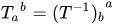
This can be thought of as a special case of a tensor with one covariant, and one contravariant index, and thus two ${\displaystyle {\mathcal {T}}}$'s are required.

All three of these symbols capture the idea of time-reversal; they differ with respect to the specific space that is being acted on: functions, vectors/spinors, or infinite-dimensional operators. The remainder of this article is not cautious to distinguish these three; the T that appears below is meant to be either ${\displaystyle {\mathsf {T}}}$ or ${\displaystyle T}$ or ${\displaystyle {\mathcal {T}},}$ depending on context, left for the reader to infer.

Eugene Wigner showed that a symmetry operation S of a Hamiltonian is represented, in quantum mechanics either by a unitary operator, S = U, or an antiunitary one ^[10], S = UK where U is unitary, and K denotes a basis-dependent complex conjugation operator. These are the only operations that act on Hilbert space so as to preserve the length of the projection of any one state-vector onto another state-vector.

For a particle with spin J, one can use the representation

$${\displaystyle T=\eta e^{-i\pi J_{y}/\hbar }K,}$$

where J_y is the y-component of the spin, and use of TJT⁻¹ = −J has been made, and ${\displaystyle \eta }$ is an arbitrary phase. ^[11]

This has an interesting consequence on the electric dipole moment (EDM) of any particle. The EDM is defined through the shift in the energy of a state when it is put in an external electric field: Δe = d·E + E·δ·E, where d is called the EDM and δ, the induced dipole moment. One important property of an EDM is that the energy shift due to it changes sign under a parity transformation. However, since d is a vector, its expectation value in a state |ψ⟩ must be proportional to ⟨ψ| J |ψ⟩, that is the expected spin. Thus, under time reversal, an invariant state must have vanishing EDM. In other words, a non-vanishing EDM signals both P and T symmetry-breaking.^[12]

Some molecules, such as water, must have EDM irrespective of whether T is a symmetry. This is correct; if a quantum system has degenerate ground states that transform into each other under parity, then time reversal need not be broken to give EDM.

Experimentally observed bounds on the electric dipole moment of the nucleon currently set stringent limits on the violation of time reversal symmetry in the strong interactions, and their modern theory: quantum chromodynamics. Then, using the CPT invariance of a relativistic quantum field theory, this puts strong bounds on strong CP violation.

Experimental bounds on the electron electric dipole moment also place limits on theories of particle physics and their parameters.^[13][14]

For T, which is an anti-unitary Z₂ symmetry generator

where Φ is a diagonal matrix of phases. As a result, U = ΦU^T and U^T = UΦ, showing that

Esto significa que las entradas en Φ son ±1, como resultado de lo cual se puede tener T ² = ±1 . Esto es específico de la antiunitaridad de T. Para un operador unitario, como la paridad , se permite cualquier fase.

A continuación, consideremos un invariante hamiltoniano bajo T. Sean | a⟩ y T | a⟩ dos estados cuánticos de la misma energía. Ahora bien, si ^T₂ = −1 , se observa que los estados son ortogonales: un resultado conocido como el teorema de Kramers . Esto implica que si T₂ = −1 , existe una degeneración doble en el estado. Este resultado en mecánica cuántica no relativista anticipa el teorema de estadística de espín de la ^teoría cuántica de campos .

Los estados cuánticos que dan representaciones unitarias de inversión temporal, es decir, tienen T 2 ⁼ 1 , se caracterizan por un número cuántico multiplicativo , a veces llamado paridad T.

La física de partículas codificó las leyes básicas de la dinámica en el Modelo Estándar . Este se formula como una teoría cuántica de campos que posee simetría CPT , es decir, las leyes son invariantes bajo la operación simultánea de inversión temporal, paridad y conjugación de carga . Sin embargo, se observa que la inversión temporal en sí misma no es una simetría (esto se suele denominar violación de CP ). Existen dos posibles orígenes de esta asimetría: uno a través de la mezcla de diferentes sabores de quarks en sus desintegraciones débiles , y el segundo a través de una violación directa de CP en las interacciones fuertes. El primero se observa en experimentos; el segundo está fuertemente restringido por la no observación del momento dipolar eléctrico ( EDM) de un neutrón .

La violación de la simetría de inversión temporal no guarda relación con la segunda ley de la termodinámica , ya que, debido a la conservación de la simetría CPT , el efecto de la inversión temporal consiste en renombrar partículas como antipartículas y viceversa . Por lo tanto, se considera que la segunda ley de la termodinámica tiene su origen en las condiciones iniciales del universo.

Strong measurements (both classical and quantum) are certainly disturbing, causing asymmetry due to the second law of thermodynamics. However, noninvasive measurements should not disturb the evolution, so they are expected to be time-symmetric. Surprisingly, it is true only in classical physics but not in quantum physics, even in a thermodynamically invariant equilibrium state.^[2] This type of asymmetry is independent of CPT symmetry but has not yet been confirmed experimentally due to extreme conditions of the checking proposal.

In 2024, experiments by the University of Toronto showed that under certain quantum conditions, photons can exhibit "negative time" behavior. When interacting with atomic clouds, photons appeared to exit the medium before entering it, indicating a negative group delay, especially near atomic resonance. Using the cross-Kerr effect, the team measured atomic excitation by observing phase shifts in a weak probe beam. The results showed that atomic excitation times varied from negative to positive, depending on the pulse width. For narrow pulses, the excitation time was approximately −0.82 times the non-post-selected excitation time (τ₀), while for broader pulses, it was around 0.54 times τ₀. These findings align with theoretical predictions and highlight the non-classical nature of quantum mechanics, opening new possibilities for quantum computing and photonics.^[15]

• El demonio de Maxwell: entropía, información, computación, editado por HSLeff y AF Rex (IOP Publishing, 1990) ISBN 0-7503-0057-4
• El demonio de Maxwell, 2: entropía, información clásica y cuántica, editado por HSLeff y AF Rex (IOP Publishing, 2003) ISBN 0-7503-0759-5
• La nueva mente del emperador: sobre ordenadores, mentes y las leyes de la física, por Roger Penrose (Oxford University Press, 2002) ISBN 0-19-286198-0
• Sozzi, M.S. (2008). Discrete symmetries and CP violation. Oxford University Press. ISBN 978-0-19-929666-8.
• Birss, R. R. (1964). Symmetry and Magnetism. John Wiley & Sons, Inc., New York.
• Multiferroic materials with time-reversal breaking optical properties
• CP violation, by I.I. Bigi and A.I. Sanda (Cambridge University Press, 2000) ISBN 0-521-44349-0
• Particle Data Group on CP violation
  • the Babar experiment in SLAC
  • the BELLE experiment in KEK
  • the KTeV experiment in Fermilab
  • the CPLEAR experiment in CERN

References

Inline citations
- ↑Veritasium (2025-04-14). The Hole In Relativity Einstein Didn't Predict. Retrieved 2025-05-31– via Emmy Noether on global and local symmetries.
- 12Bednorz, Adam; Franke, Kurt; Belzig, Wolfgang (February 2013). "Noninvasiveness and time symmetry of weak measurements". New Journal of Physics. 15 (2) 023043. arXiv:1108.1305. Bibcode:2013NJPh...15b3043B. doi:10.1088/1367-2630/15/2/023043. S2CID 17583996.
- ↑Kubo, Ryogo (15 June 1957). "Statistical-Mechanical Theory of Irreversible Processes. I. General Theory and Simple Applications to Magnetic and Conduction Problems". Journal of the Physical Society of Japan. 12 (6): 570–586. Bibcode:1957JPSJ...12..570K. doi:10.1143/JPSJ.12.570.
- ↑Bonella, Sara; Ciccotti, Giovanni; Rondoni, Lamberto (2015). "Time reversal symmetry in time-dependent correlation functions for systems in a constant magnetic field". EPL (Europhysics Letters). 108 (6) 60004. doi:10.1209/0295-5075/108/60004. S2CID 121427119.
- ↑Luo, Rongxiang; Benenti, Giuliano; Casati, Giulio; Wang, Jiao (2020). "Onsager reciprocal relations with broken time-reversal symmetry". Physical Review Research. 2 (2) 022009. Bibcode:2020PhRvR...2b2009L. doi:10.1103/PhysRevResearch.2.022009.
- ↑Carbone, Davide; Rondoni, Lamberto (2020). "Necessary and sufficient conditions for time reversal symmetry in presence of magnetic fields". Symmetry. 12 (8): 1336. arXiv:2008.05193. Bibcode:2020Symm...12.1336C. doi:10.3390/sym12081336.
- ↑Kerdcharoen, Teerakiat; Liedl, Klaus R.; Rode, Bernd M. (1996). "Bidirectional molecular dynamics: Interpretation in terms of a modern formulation of classical mechanics". Journal of Computational Chemistry. 17 (13): 1564–1570. doi:10.1002/(SICI)1096-987X(199610)17:13<1564::AID-JCC8>3.0.CO;2-Q.
- ↑Chakhmakhchyan, Levon; Cerf, Nicolas (2017). "Boson sampling with Gaussian measurements". Physical Review A. 96 (3) 032326. arXiv:1705.05299. Bibcode:2017PhRvA..96c2326C. doi:10.1103/PhysRevA.96.032326. S2CID 119431211.
- ↑ Chakhmakhchyan, Levon; Cerf, Nicolas (2018). "Simulación de circuitos gaussianos arbitrarios con óptica lineal". Physical Review A . 98 (6) 062314. arXiv : 1803.11534 . Bibcode : 2018PhRvA..98f2314C . doi : 10.1103/PhysRevA.98.062314 . S2CID 119227039 .
- ^ Wigner, Eugene Paul (1931). Gruppentheorie und ihre Anwendung auf die Quantenmechanik der Atomspektren (en alemán). Braunschweig: F. Vieweg und Sohn.
- ^ Wigner, Eugene Paul (1931). Gruppentheorie und ihre Anwendung auf die Quantenmechanik der Atomspektren (en alemán). Braunschweig: F. Vieweg und Sohn. pag. 282.
- ↑ Khriplovich, Iosip B.; Lamoreaux, Steve K. (2012). Violación de CP sin extrañeza: momentos dipolares eléctricos de partículas, átomos y moléculas . [Sl]: Springer. ISBN 978-3-642-64577-8.
- ↑ Ibrahim, Tarik; Itani, Ahmad; Nath, Pran (12 de agosto de 2014). "Electron EDM as a Sensitive Probe of PeV Scale Physics". Physical Review D . 90 (5) 055006. arXiv : 1406.0083 . Bibcode : 2014PhRvD..90e5006I . doi : 10.1103/PhysRevD.90.055006 . S2CID 118880896 .
- ↑ Kim, Jihn E.; Carosi, Gianpaolo (4 de marzo de 2010). "Axiones y el problema CP fuerte". Reviews of Modern Physics . 82 (1): 557– 602. arXiv : 0807.3125 . Bibcode : 2010RvMP...82..557K . doi : 10.1103/RevModPhys.82.557 .
- ↑ Angulo, Daniela; Thompson, Kyle; Nixon, Vida-Michelle; Jiao, Andy; Wiseman, Howard M.; Steinberg, Aephraim M. (2024). "Evidencia experimental de que un fotón puede pasar una cantidad negativa de tiempo en una nube de átomos". arXiv : 2409.03680 [ quant-ph ].
Referencias generales